IF YOU HAVE
PROBLEMS ACCESSING
LINKS STARTING WITH-
http://www.mae.ufl.edu/~uhk/*
TRY INSTEAD-
http://www2.mae.ufl.edu/~uhk/*

 THE
STATICS PAGE
THE
STATICS PAGE

"The most valuable of
all
talents
is that of never using two words where one will do"-Thomas
Jefferson
(1743-1826)
I am revising and updating our earlier Statics
Page
and presenting the results below for our Class EGM
2511. You can use it to gain further
insight
into the basic concepts of statics. Also it contains extra
information
of use to you such as what topics are to be discussed in
upcoming
lectures. The book we are using is the
9th
edition of ENGINEERING
MECHANICS-STATICS
by
R.C.Hibbeler. It is easy to read and understand and
free of
errors. The knight on horseback points to the next lecture. If
you
have questions please contact me at kurzweg@ufl.edu
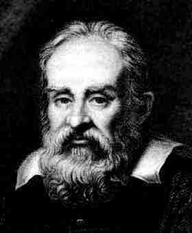
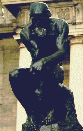
Do you recognize the
three
photos
above? They are of Galileo Galilei (1564-1642) and Sir Isaac
Newton
(1643-1727)
the two most important early contributors to classical
mechanics , and
the statue of the Thinker by Rodin(about 1910)
located in
Paris.
LECTURE #1:-Introductory
remarks,
Newton's three laws of motion, plus the universal
gravitational
law, SI and US systems of units.
LECTURE#2:-
Properties of vectors, Forces as vectors,Vector addition ,
subtraction
and multiplication, Position vectors.
SOME INTERESTING
CONVERSIONS
AND LENGTH SCALES: A few helpful conversions are: 1
inch=2.540cm,
1 km=0.6215mile, 1 lb=4.448N, 1 slug=14.593kg, 1 ft-lb=1.3558
joules, 1
hp= 550 ft-lb/sec=745.70 watts(or joules/sec), 1 mile/hr=
1.6093 km/hr,
and 1 lb/in^2=6894.76 pascal. While we're at it-
One Light Year=186,000
miles/sec
x 3600 sec/hr x (24 x 365) hr/yr=5.87x10^12
miles=9.46x10^12km
The diameter of our
galaxy(
Milky
Way) is about 100,000 light years , the sun is 500 light
seconds away
from
the earth, the next nearest star (Alpha Centauri) is 4.3
light years
away,
and we can see out a distance of between 9 and 18 billion
light years
with
the best optical and radio telescopes. Radiation coming from
this last
distance started its journey 18 billion years ago at the
beginning of
the
universe( big bang theory). If you want some really small
distances try
1 micron=10^-6 meter for the size of a typical microchip
structure,
0.529
angstrom=0.529x10^-10 meter for the radius of the first Bohr
orbit of
the
hydrogen atom , and 2.4x10^-15 meter for the diameter of a
proton. The
web has available many convenient sites for converting
between SI and
US
Customary
units.
CLIMB ANGLES AT THE
GREAT
PYRAMID:To
demonstrate the use of vectors in carrying out certain
geometrical
calculations,
we were asking in class what are the angles associated with
climbing
the
great pyramid of Cheops at Giza in Egypt. One can look up on
the
internet
that the base of this pyramid has sides of length b=756 ft .
The four
sides
of this pyramid are in the form of equilateral triangles.
Placing the
origin
of a cartesian coordinate system at the center of the base,
it is easy
to show that the coordinate of the pyramid vertex is at
(0,0,b/sqrt(2)).
Thus the position vector of length b running along one of
its edges is
R=-bi/2-bj/2+bk/sqrt(2). Taking a dot product of this vector
with k
yields
cos(theta)=1/sqrt(2), or a climb angle of 45 deg. Note that
the climb
angle
starting from the middle of one of the sides is much steeper
and equals
54.73 deg. , again shown by dot product manipulations. If
you ever get
a chance to go over there sometime you will be truly amazed
at this
engineering
marvel of the ancient world. They don't let you climb the
pyramids of
Giza
anymore but you can go inside those of Cheops and Cephren
(as I
remember
doing back in 1983) .
LECTURE#3:-More
on Forces, Equlibrium of a particle in 2D , Concept of unit
vectors
along
a given direction.
LECTURE#4:-3D
Equilibrium Problems. Working out in detail several equilibrium
problems
from the book.
LECTURE#5:-Concept
of a Couple. Working out several more problems in static
equilibrium.
WHAT ARE MOMENTS AND
COUPLES?:A
moment M is defined as the cross product between a position
vector from
the point about which the moment is taken and a force F,
that is M=rxF.
The simplest way to evaluate this product is via a three by
three
determinant
in which the first row elements are the base vectors i,j and
k. The
second
row consists of the position vector components and the third
row are
the
force components. Thus r=2i+5j-3k and F=20i-40j+30k yields
M=30i-120j-180k.
The dimensions of M are length-force and so given in ft-lb
in the US
system
of units and in met-newton in SI. A couple C consists of two
equal but
opposite forces F and -F separated by a position vector r.
The couples
value is simply rxF and will retain this same value no
matter about
which
point the moments for the two forces are taken. The couple
produced by
F=10j acting at (3,0,0) and -F=-10j acting at (-3,0,0)is
C=60k.
LECTURE#6:-Completion
of the combined couple, moment and force problem acting on a
2D slab.
Several additional
problems
from the book worked out in detail.
BASIC LAWS OF STATICS: We
have now reached the point in the course where we can state
the basic
Laws
of Static Equilibrium and the rest of the course will be their
application
to all sorts of problems, which, as you will find, is not
always that
easy.
The Laws are-
(1)-THE SUM OF ALL FORCES
ACTING
ON A BODY IN STATIC EQUILIBRIUM MUST BE ZERO.
(2)-THE SUM OF ALL
MOMENTS(INCLUDING
COUPLES) ACTING ABOUT ANY POINT ON THE BODY MUST BE ZERO.
LECTURE#7:-Component
of a moment about a given line. Examples worked out in
detail.
MOMENT ABOUT A SPECIFIED
LINE
IN SPACE:-In solving some statics
equlibrium
problems one can often determine an unknown force(such as a
tension in
a rope attached to the body) by taking moments about a line
passing
through
two points on the body at which there exist other unknown
forces . By
so
doing you avoid having to solve for these other forces. To
carry out
this
procedure requires knowledge of the moment about such a line.
Let me
demonstrate
how this is done. Consider a cube extending over the range
0<x<1,0<y<1,0<z<1
. A force F1=10i+20j-30k acts at corner(x=1,y=0,z=1)and a
second force
F2=-10i+40k acts at corner (1,1,1). The moment produced by
these two
forces
about the origin at (0,0,0) is
M=(i+k)x(10i+20j-30k)+(i+j+k)x(-10i+40k)=20i-10j+30k.
Now lets ask what is the projection of this moment on a line
connecting
the origin (0,0,0) and (1,1,0). We have this line defined by
the unit
vector
u=(i+j)/sqrt(2) so that dotting it with M yields 10/sqrt(2).
Thus the
moment
about the line becomes 5i+5j. Run through this calculation
yourself
using
a sketch and also see if you can get this result another way.
Note that
we took the original moment about a point on the line chosen.
Would you
be able to obtain a moment projection along a given line if
the
original
moment is taken about a point not on the line?
LECTURE#8:-Reduction
of Force and Couple Systems. Concurrent, Coplanar, and
Parallel
Force
Systems. The Wrench. Location of Resultant Forces.
EQUIVALENT FORCE SYSTEMS:
In many statics problem involving the effect of several forces
acting
on
a body, it is often convenient to replace these with a single
resultant
force plus a couple, before proceding further in the
calculations. To
show
you how one can establish such an equivalent system, look at the
simple
example HERE.
LECTURE#9:-Free
Body Diagrams . Forces and Moments acting at different Supports
. Pins,
Rollers, Rockers, Hinges, plus Ball and Socket Joints.
HOW TO HANDLE DISTRIBUTED
FORCES:
When dealing with continous force distributions on extended
bodies it
is
convenient to replace these with a single resultant force R
acting at a
given point P. To see how one determines the value of the
equivalent
force
and its location, we consider the case of a weighless
horizontal beam
of
length x=L which is loaded by a distributed downward linear
force
distribution
w(x)=a+bx (expressed in force per length) and supported
at end
points
at A and B. In this case the moment about the z axis produced
by this
distributed
force about the left pivot point at A has magnitude
M=-Int[xw(x)dx]=-[(1/2)aL^2+(1/3)bL^3].
In static equilibrium this plus LBy, where By is the vertical
force on
the beam at the right support, must be zero. Hence the
resultant
downward
force R=Int[w(x)dx] acts at a distance x*=LBy/R. This turns
out to be
at
x*=L[(a/2+bL/3)/(a+bL/2)] for this linear force distribution
and thus
at(
/3)L when a=0. Click HEREto
see a picture of the configuration.
LECTURE#10:-Working
out more Statics problems in 2D and 3D for all sorts of
different
supports.
Don't
forget about your First Statics Exam coming
up next week.
LECTURE#11:-Working
out
more statics problems in 2D and 3D from Chapter 5.
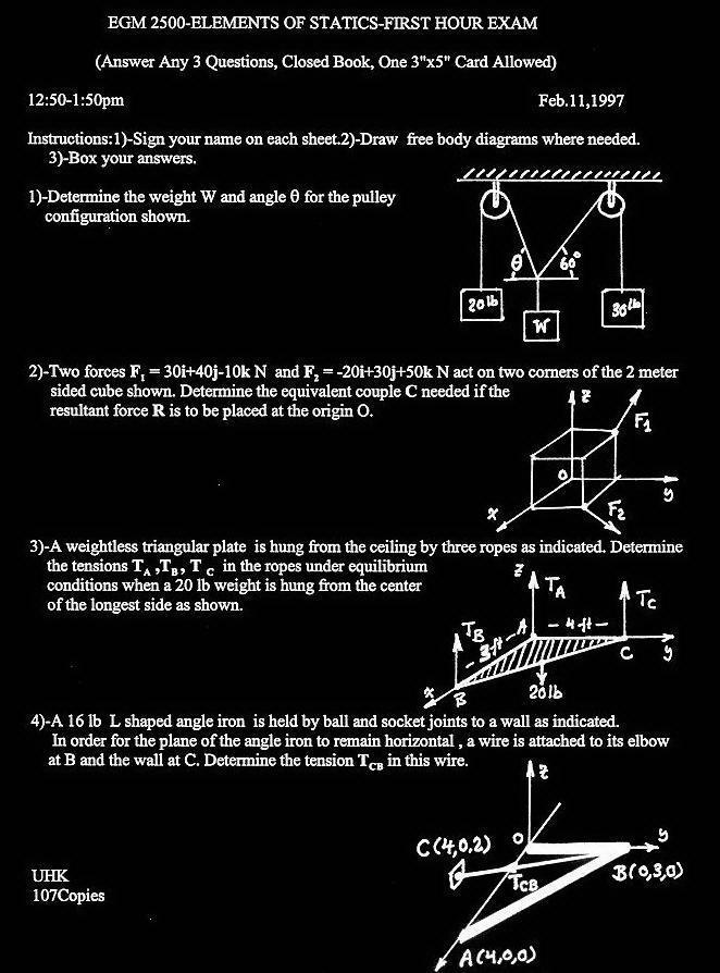
Some of you have asked me about posing an old
#1
exam. Here
is one from 1997 which you can use to practice and get up to
speed .
STACKING OF BRICKS TO FORM
A
STATICALLY STABLE ARCH: Every
once in a
while
one discovers certain facinating problems even in topics as
elementary
as statics. One of these I ran across this weekend is an
extention of
solving
the problem of the furthest distance three bricks
stacked on top
of each other can have their centers of gravity moved to the
right
without
causing the pile to tumble. The three brick problem is easy to
solve .
It is clear from a moment balance that the second brick can be
moved a
half brick length to the right of the top brick without
falling. Next
the
two bricks in the top two rows have their center of gravity at
1/4 of a
brick length so that the bottom brick can be placed at 3/4 of
a brick
length
to the right of the top brick. Now comes the interesting
extention.
Consider
n rows containing one brick each. Again starting with the top
row, the
next to the top row is placed at 1/2 to the right for a unit
length
brick.
The one after that is at 3/4. Continuing on, we find the brick
in the
n+1
row from the top is at x[n+1]=x[n]+1/(2n)
with x[1]=0, x[2]=1/2, x[3]=3/4, x[4]=11/12, x[5]=25/24, etc.
Using the
canned program MAPLE to evaluate this for a 20 row stack, we
find the
result
shown HERE.
This
result looks very much like half of a parabolic arch and becomes
a full
arch when we also allow the same type of stacking on the other
side .
Note
that you wouldn't need any binder to build such an arch.
Undoubtably
such
stacking by early man is how he first came up with the idea of
the
arch.
It is interesting to note that the ancient Greeks did not
use a
proper
arch in their architecture* and
that it
was
not until Roman times that the circular arch was invented and
used in
bridge
and building construction. The arch reached its high point
during the
midle
ages with the discovery of the gothic arch. This last structure,
when
used
in conjunction with a flying buttress, is extremely stable since
all
compression
loads lie strictly along the arch and accounts for the fact that
many
of
the European cathederals have remained intact for nearly a
thousand
years.
*-Several years ago
I
visited an ancient tomb in Mycenae in Greece built some 3000
years ago.
The tomb has an entrance arch formed by stacking up stone
plates, but
making
the overlap the same for all rows. In view of the problem solved
above,
you can see why this was not the best solution and not really a
true
arch.
REVIEW
FOR THE FIRST EXAM. The exam will be closed book and
cover
chapters 1 through 5. You can answer any three of the four
questions.
Lecture #12:-Structural
Analysis(beginning of Chapter 6). Simple Trusses.
Concept of
Compression
and Tension in Members. Method of Joints.
ANALYSIS OF A TRUSS: We
have shown in class that the concatenation of triangular
shapes formed
by three members connected at their ends produces a stable
truss which
is the basic building block for most structures be they roof
trusses,
railroad
bridges , furniture, etc. In the analysis of such structures
one first
solves for all the external forces acting on the truss and
then looks
at
the internal forces by either the method of joints or method
of
sections.
We give HERE
a very simple example of such an analysis. The important thing
to
remember
is that the internal forces produce a compression
in
a member when the calculated force points toward the pin at
the joint.
When your calulations show the force going away from the pin
then the
member
is in tension.(just
the opposite of what a cursory glance would suggest)
Lecture#13:-More
on Trusses. The Crane Problem. Method of Sections.
Lecture #14:-Completion
of
discussion on trusses in 2D by application of both the Method of
Joints
and the Method of Sections.
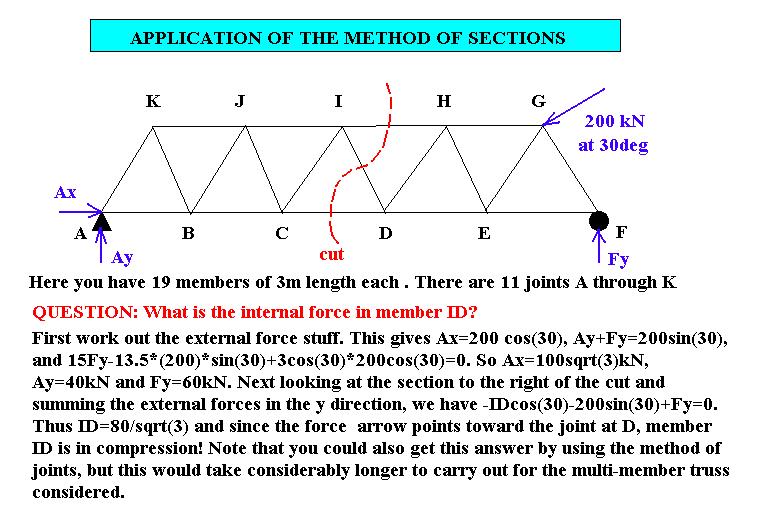
APPLICATION OF THE
METHOD
OF
SECTIONS: When one is
interested in just
one
of the internal forces of a member of a truss, especially
when the
truss
has many members, it is convenient to use the method
of sections. This involves
putting a cut
through
the truss including the member in whose internal force we
are
interested.
Next treating the unknown forces in the cut members as
external forces,
one can rapidly find the value of the force in the member
and generally
can do so much faster than when using the method of joints.
We
demonstrate
this solution method for one particular truss HERE.
Have
you ever wondered how many members M and joints J a truss
composed of N
triangles has? You can arrive at a relation between these
three
quantities
by slowly working up from N=1. Thus when N=2 you have M=5 and
J=4. Next
for N=3 you find M=7 and J=5. Continuing on, you soon realize
that J=N+2
and
M=2N+1. Thus a truss with 80
triangle
components
will have 161 members and 82 joints.
Lecture #15: Trusses
in 3D(Space Trusses). Introduction to Frames.
THE "A" FRAME: A
prime
example of a frame stuctrure is the A frame used in a variety of
structures
including tables and vacation homes. it consists of two two side
legs
plus
one cross bar anchored together by pins at the three joints. You
analyze
a problem of this type by looking at the three members
individually
after
determining the external reactions on the frame. If you go HERE
you will see the analysis when the members are weightless and a
weight
W is hung from the center of the cross-bar. Note how one always
reverses
the forces at a joint in going from one member to the other. If
you
should
assume the wrong direction of the force at a joint, this will
come
clearly
at the end of the calculations by giving you a minus sign.
Lecture #16:
More on Frames and Machines. The Crank-Piston Problem. Analysis
of
multiple
pulley systems.
ANALYSIS OF A PULLEY:
We all learned back in high school physics that there are six
simple
machines,
namely, (1)the lever, (2)the screw, (3)the wheel and axle,
(4)the
wedge,
(5)the inclined plane, and (6)the pulley. Of these , the pulley
is
usually
the one hardest to understand. In view of our discussion on
machines it
is actually quite easy to grasp by analyzing each wheel
sub-section
individually
as shown HERE.
At wheel A we see, via a vertical force balance,(assuming
negligible
weight
of the wheel) that the force in the rope going about the wheel
is equal
to F while the rope holding wheel A has a tension of 2F. going
on to
wheel
B we see that the rope hung from the wheel axis must be 2F by a
force
balance.
Continnuing this analysis on through wheel D, one sees that it
can
carry
a weight of 8F. By using n wheels in such a pulley the
mechanical
advantage
gained will be 2^(n-1). That is, one could use such a pulley to
lift a
640lb car engine with a force of just F=40lb, when the pulley
has five
wheels.
Lecture #17:
Completion
of discussion on Frames and Machines, plus Introduction to
Internal
Forces(Chapter
7).
Drawing Shear and Bending
Moment
Diagrams: The basic formula for determining shear in a
1D beam
is
dV/dx=-w(x), where w(x) is the x dependent downward loading and
V is
the
shear. The shear is thus a constant where the loading is zero
and will
vary linearly with x for constant loading. The bending moment
formula
is
dM/dx=V(x), with M vanishing at the end supports(except at those
which
can sustain a moment such as a cantilever). Note that if V is a
polynomial
of order n then the bending moment M will be one of order n+1 .
The
jump
in V at a point load is just equal to the value of this load. By
clicking
HERE
you can see a typical example of a shear(orange) and bending
moment(blue)
diagram for a cantilever beam subjected to a linearly varying
load.
Lecture #18-Working
out Shear and Bending Moment Diagrams for a variety of
different
loadings.
No classes next week due to
spring break. Enjoy the vacation!
Lecture #19-More
on Shear and Bending Moment Diagrams. Also Shear and Normal
Force in
Curved
Beams.
N,V, AND M FOR A CURVED
BEAM:-So
far we have looked at normal (N) and shear(V) forces
plus the
bending
moments(M) in only 1D beams for which the simple formulas
dV/dx=-w(x)
and
dM/dx=V(x) apply. Let us next extend the discussion to curved
beams.
Take
the case of a weightless semicircular beam of radius r=a
pushed against
a smooth floor by a single force Fo applied at its
top as
shown
HERE.
The analysis proceeds as usual by first determining the
external
forces.
These are simply Ay=By=Fo/2.
To now
find
N, V, and M at some point C along the curved beam, we apply to
the beam
segment B-C the conditions that the summation of forces in the
x and y
direction are zero and that the sum of the moments taken
at C
must
also be zero . A simple calculation then yields V=-(Fo/2)sin(q),
N=(Fo/2)cos(q) and M=(aFo/2)[1-cos(q)],
in the range 0<q<p/2. For p/2<q<p
we
have a change in sign for V and the bending moment becomes M=(aFo/2)[1+cos(q)].
Note the maximum bending moment occurs at the top of the
semicircle
where
q=p/2
and vanishes where the semicircle touches the floor.
Lecture #20: Completion
of stuff on Shear and Bending Moments. How to handle a hook
input. Also
a discussion on Cables and the Shape of a Suspension Bridge
Cable.
Shape of a Suspension
Bridge
Cable: In discussing cables during the previous lecture
we asked
the question what would be the shape of a cable of if it is
subjected
to
a uniform x dependent loading w(x)=Const. This is the well
known
suspension bridge problem which predicts, as shown HERE,
that the shape of the cable is that of a parabola
y=const x2. Note that a cable hanging under
its own
weight
has a different shape , namely, that of a catenary curve
y=cosh(a*x).
Lecture #21: Introduction
to Coulomb Friction. Angle of Repose and Problem of
Ladder
Equilibrium
when resting on a rough floor.
Lecture #22:
More
on Dry Friction including discussion of the Wedge Problem.
Lecture #23: Belt
Friction, Tipping and Sliding.
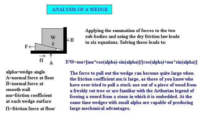
THE WEDGE PROBLEM:
One
of the problems which can be well explained by using Coulomb's
friction
law f=mN is that of the wedge.
Consider a
wedge
with wedge angle a used to hold up
a weight
W as shown HERE.
The external forces acting are indicated and we are
particularly
interested in determining the ratio of F/W as a function of m
and a
, where the coefficient of friction at
the wall is zero but has the same value of m
on
both wedge surfaces. Looking at the system as two bodies with
friction
forces f1 and f2 parallel to the two wedge surfaces, one finds
a total
of six equations governing equilibrium which can be solved to
find F,
A,
B, f1, f2, and alpha for a given weight W and friction
coefficient
m.
We have neglected the wedge weight w in our calulations since
typically
W>>w.
Lecture #24:
Completion
of discussion on dry friction by working some problems from the
book.
BELT FRICTION:
When you wrap a rope about the circumference of a cylinder,
one
typically
finds that there is a difference in the rope tension at the
two points
where the rope leaves the cylinder. This tension difference is
due to
friction
effects and can become quite large when wrapping the
rope
multiple
times around the cyliner. The equation for the tension change
is T=Toexp(mq),
where m is the coefficient of
friction
between
the rope and the cylinder surface and q
the
total angle the rope is wrapped around the cylinder. Since the
exponential
term is greater than unity, it is clear that T>To. This
means that the friction force f will always be opposite
to the
direction
of impending motion. Go HERE
to see the derivation of the belt friction equation. Such belt
friction
is employeed by capstans used to tie up large boats at harbour
docks
and
in devices for slowly lowering heavy weights.
REVIEW FOR
SECOND
HOUR EXAM: Same format as
exam #1
Lecture #25:
Beginning of Chapter 9 on Center of Gravity and Centroids.
Basic
definitions
and use of calculus to find CGs for various 2D and 3D
bodies.
Lecture #26: Centroids
and
CGs for Composite Bodies.
CENTROID OF COMPOSITE
BODIES
WITH HOLES: We have shown in
class how the
centroid of a 2D composite body is calculated by looking at
the
quotient
of the sum of the products of xbar and the sub-area divided by
the
total
area. When a body contains a hole the procedure stays the same
except
that
the sub-area representing the hole is preceded by a negative
sign. To
demonstrate,
take the circular disc x^2+y^2=4 into which is cut a square
hole
0<x<1,
-1/2<y<1/2. Here by symmetry ybar is zero but xbar
becomes
[0*4*Pi-0.5*1]/[4*Pi-1]=
-0.043228. So xbar is negative as expected. Click HERE
to see a schematic of this calculation.
CENTROID FOR A COMPOSITE
BODY:
To get some practice on finding the centroid of some 2D
systems,
consider
the centroid of the block letter combination UF ( University
of Florida
).What is x bar and y bar for this set up assuming both
letters U and F
are constructed of unit width rectangles and the two letters
are
separated
by a unit distance? To make the calculation we break the U up
into
three
rectangles. The first of these has corners at (-4,5),
(-4,0),(-3,0)
and(-3,5).
The second has corners at (-3,0), (-1,0), (-1,1) and (-3,1)
and the
third
corners at (-1,0), (0,0), (0,5) and (-1,5). Applying our
composite body
formula to these three rectangles yields a centroid for the U
of
xbarU=[xbarI*AI+xbarII*AII+xbarIII*AIII]/[AI+AII+AIII]=-2.00
and
ybarU=[ybarI*AI+ybarII*AII+ybarIII*AIII]/[AI+AII+AIII]=13/6.
Thus
the
centroid of U is at (-2.00,2.1667). Next look at F. Breaking
it also up
into three rectangles with the largest having corners at
(1,0),(2,0),(2,5)and(1,5).
The other rectangle has corners at (2,4), (5,4), (5,5) and
(2,5) with
the
remaining square bounded by corners (2,2), (3,2), (3,3) and
(2,3). One
finds for the F the centroid is at (xbarF,
ybarF)=(2.2778,3.16667).
Finally
combining the centroids for U and F yields
xbar=[-2*12+(41/18)*9]/[12+9]=-0.1667
and ybar=[2.2778*12+3.16667*9]/21=2.5952. Thus the UF
combination will
have zero net moment about the point (-0.16667, 2.5952). I
gave this
problem
several years ago as one of the problems on a statics exam
and, if I
remember
correctly , about half got it right.
Lecture #27: More
calculations for the CG and Centroid of Bodies plus the
Theorems of
Pappus
and Guldinus.
THEOREMS OF PAPPUS
AND
GULDINUS: There
are two theorems associated with the the names of Pappus of
Alexandria(
290-350AD) and Guldinus( 1577-1643AD). The first of these
states that
"the
product of the length of a curve and the distance moved by
its centroid
when the curve is rotated about an axis equals the surface
area
generated".
As an example consider the half circle x^2+y^2=R^2, y>0.
Its length
is
R*Pi and its centroid is at 2*R/Pi. Thus by the first
theorem the
surface
area will be R*Pi*(2*Pi)*(2*R/Pi)=4*Pi*R^2, a well known
result from
calculus.
Use this theorem to calculate the surface area of a toroid.
The second
theorem states that "The product of an area and the distance
travelled
by its centroid when this area is rotated about an axis
equals the
volume
of the solid generated". As a demonstration of this consider
the
rectangle
-a<x<a, 0<y<b rotated about the x axis. Its area
is 2ab and
its ybar is b/2. The volume generated is thus V=2a*b^2*Pi.
This agrees,
as expected, with the volume of a cylinder of height 2a and
radius b.
Go HERE for a
derivation of
the Pappus Theorems.
Lecture #28:
Resultants
for Distributed Loadings. Fluid Pressure, Pascal's Law
and Center
of Pressure.
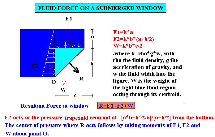
FORCE ON SUBMERGED
SURFACES:
The centroid concept can be applied to loading of surfaces due
to
hydrodynamic
forces. Click HERE
to
see the general development for the resultant force on a
submerged
window.
Also consider the case of the resultant force R on a vertical
dam of
height
h and width w. By Pascal's law we know the fluid pressure at
depth z
will
be p=rgz so the force on the dam
will be R=Int[rgz
dz,
z=0..h]=rgwh2/2.
That is, the force equals the dam area w*h times the average
hydrostatic
pressure rgh/2. Note, R is
not
dependent
on how much water is stored behind the dam. On the other
hand, R
becomes
very large for dams such as the Hoover dam in Nevada where
h=725ft.
Note
the resultant force R acts at the center of pressure which
lies at the
centroid of the pressure triangle and thus at h/3 from the
bottom for a
filled , vertical walled, dam.
Lecture #29: Introduction
to Moments of Inertia(Chapter 10). Basic definition and
parallel axis
theorem.
Using calculus to find Ixx, Iyy, and Izz.
Go HERE to see how
calculus
is used to determine these for various bodies.
AREA MOMENTS OF
INERTIA
FOR
A RECTANGULAR PLATE: A good
demonstration
of area moments of inertia is given by looking at the
rectangular plate
0<x<a, 0<y<b. In this case the values Ixx=Int[y^2dA]=a*b3/3
and
Iyy=Int[x^2dA]=b*a3/3. Also Izz=Jo=Int[r2dA]=Ixx+Iyy=[(a*b)/3]*[b2+a2].
This
last relation between the three area moments of inertia holds
only
for lamina and is often referred to as the perpendicular
axis theorem. We also have from
the parallel
axis theorem that the Izz
will
have its minimum value at the plate centroid at x=a/2, y=b/2.
The
explicit
value is Izz(at lower left corner)=Izz(at
plate
centroid)+(plate
area)*(square of the distance between the two points).
Here this yields Izz(at plate centroid)=(a*b/12)*(a2+b2)
which is seen to be four times less than that about any of the
plate's
corners. Note the area moments of inertia have the
dimension of
length to the 4th power, while mass moments of inertia have
dimensions
of mass times length squared.
Lecture #30:
Moments of Inertia of Composite Bodies.
AREA MOMENT OF INERTIA FOR
A
COMPOSITE LAMINA: Moments of
inertia are
additive
so that one can readily calculate the I values of a composite
body
about
any chosen axis by knowing the values for the sub-bodies and
then
applying
the parallel axis theorem. HERE
is an example of such a calculation.
Lecture #31:
Product of Inertia Ixy, Moment of Inertia about any
Axis,
Principal
Moments of Inertia, Mohr Circle.
MOMENT OF INERTIA ABOUT AN
ARBITRARY
AXIS IN THE PLANE OF A LAMINA:
Consider a
lamina with a superimposed x and y axis. Introduce a second
pair of
orthogonal
axis u and v where the u axis makes an angle of A with respect
to the x
axis. From the geometry it is easy to express u and v as
functions of x
and y , as we have done in class, and then work out the area
moments of
inertia Iuu and Ivv, plus the product of inertia Iuv. Go HEREto
see the details. Note also the Mohr Circle follows from this
analysis.
Lecture #32:
Mass Moments of Inertia defined and evaluated using Calculus.
Radius of
Gyration.
CALCULATING THE MASS MOMENT
OF INERTIA FOR A UNIFORM SPHERE:
We have
defined
the mass moment of inertia about the z axis of a body as
Izz=Int[(x^2+y^2)*dm],
where the integral extends over the entire body with the mass
increment
dm=rho*dxdydz. In many cases one does not need to carry out
the
integration
of such triple integrals directly if one knows the value of
dIzz of the
sub-bodies making up the body of interest. We show you HEREthe
calculation for finding Izz of a uniform sphere of radius R=a
using the
known dIzz for the discs making up this sphere.
Lecture #33:-Concept
of
Virtual Work(Chapter 11)and some Elementary
Applications.
EXAMPLE OF A VIRTUAL WORK
PROBLEM:
We
have shown in class that an alternative method for solving
static
equilibrium
problems is that of Virtual Work. The technique is based on
the fact
that
the product of the forces acting on a body times their virtual
displacements
must add up to zero under static equlibrium. The virtual work
will be
W=F.dr
and applies only to those points where the force F can cause
virtual
displacements
dr. We show you
HEREa
simple application.
Lecture #34:-
More
on Virtual work. Conservative Forces, and Potential Energy. Also
filling out of teacher and course evaluation forms for Dr.
Kurzweg's
section
1576.
SMALL
SIDE DIVERSION ON PI
 REVIEW
FOR THIRD EXAM : This exam
will emphasize Chapters 9, 10
and
11 on Centroids, Center of Gravity, Moments of Inertia, and
Virtual
Work.
One of the problems will also contain material (such as possibly
frames
and friction)covered in the earlier chapters.
REVIEW
FOR THIRD EXAM : This exam
will emphasize Chapters 9, 10
and
11 on Centroids, Center of Gravity, Moments of Inertia, and
Virtual
Work.
One of the problems will also contain material (such as possibly
frames
and friction)covered in the earlier chapters.
November 27, 2010
