![]()
INTRODUCTION: Over the past thirty five years I have taught an introductory sequence of graduate level courses in mathematical analysis for engineering majors. An estimated 3000 students have attended these courses and the topics covered are Advanced Ordinary Differential Equations (EGM6321), Partial Differential Equations and Boundary Value Problems(EGM6222), and Integral Equations and Variational Methods(EGM6323). We present here a collection of equations and graphs for the various mathematical functions encountered in our lectures and give some relevant historical information on the mathematicians associated with their discovery. Equations and figures are presented in sequential order as they arise in the lectures. You can view the graphs by clicking on the underlined titles or the activated word HERE. The graphs have been generated by a variety of canned programs including Maple, Matlab, Mathematica, and Mathcad. OUTLINES for the three courses are found HERE, HERE,andHERE. In the descriptions below we are using a type of mathematical esperanto since html does not have the standard math symbols in its repertoire.
You can contact me at E-Mail kurzweg@ufl.edu or reach me via standard mail at U.H.Kurzweg, MAE-A Bldg, University of Florida, Gainesville, FL 32611, USA. This page is found on the internet at http://www2.mae.ufl.edu/~uhk/MATHFUNC.htm
In case you are wondering what an image
of Duerer's etching "Melancholia" is doing on our title
page? It's mainly due to the 4x4 magic square shown above the
head of the seated thinker. Known as Duerer's magic square ,
its matrix reads [16,3,2,13;5,10,11,8;9,6,7,12;4,15, 14,1]
with the semicolons separating rows. Note that the
juxtaposition of elements a4,2=15 and a4,3=14
in the fourth row give the 1514 completion date of the
etching. The numbers along any vertical, horizontal or
diagonal line in his magic square add up to n(n^2+1)/2=34,
which when read backwards gives the artist's age at the time
of the etching. Duerer the artist (1471-1528) obviously also
had more than just a cursory interest in mathematics and
numerology!
At
the
bottom of this WEB page you will also find some of our latest thoughts and discussions
on additional mathematical subjects of common
interest not covered directly by our three analysis courses.
They appear in chronological order with the latest at the
end. Some of these topics might be of interest to the
readers as they contain a lot of new and original
observations of possible use for
future studies especially in the area of number theory.

EGM 6321-ADVANCED ORDINARY DIFFERENTIAL EQUATIONS
Solution of linear and non-linear ordinary differential
equations. Method of Frobenius, classification of singularities.
Integral representations of solutions. Treatment of the Bessel,
Hermite, Legendre, Hypergeometric and Mathieu
equations. Asymptotic methods including the WBK and saddle
point techniques. Treatment of non-linear autonomous
equations. Phase plane trajectories and limit cycles.
Thomas-Fermi, Emden, and van der Pol equations.
ISOCLINE SOLUTION OF FIRST ORDER ODE'S: - There is available on the WEB a numerical program written by John Polking for MATLAB ( http://math.rice.edu/~dfield/) which can draw isoclines for the solution of any first order ODE and then allow one to graph the solution curve which satisfies a particular initial condition. I demonstrate the use of this program for the deceptively simple equation y'=1/x-1/y which clearly has solutions with infinite slope along both the y and x axis. Can anyone find an analytic solution to this equation? I've been waiting for one for ten years.
THE LOGISTIC EQUATION: -One of the better known first order ODE's is the logistic equation y'=y(1-y) which arises in describing population growth of a species in an environment with limited resources and also arises in connection with certain studies in chaos. It is a special case of the Bernoulli equation y'+p(x)*y=q(x)*y^n and has a straight forward separation of variables solution y=1/[1+((1-A)/A))exp(-x)] , where y(0)=A and y(infinity)=1. We give here the graphs of this solution and its isoclines for several different initial conditions A.
OBLIQUE TRAJECTORIES:- Consider a family of curves defined by the first order differential equation y'=f(x,y). Now think of a second family of curves which intersect these curves at angle a. These later curves are referred to as the oblique trajectories and they have the slope y'=(f+m)/(1-f*m) as is readily established by use of the double angle formula for tangent. The constant m=tan(a). Consider now the case of the oblique trajectories intersecting the concentric circles x^2+y^2=C^2 at 45 degrees. Here f=-x/y and m=-1, so that the governing equation for the trajectories becomes y'=(x+y)/(x-y). This is a homogeneous equation solvable by the variable substitution v=y/x and yields the logarithmic spiral which (in polar coordinates) reads ln(r)=[A+B*q]. A plot of one of these spirals for A=0 and B=1 is shown in the accompanying graph. The famous mathematician Jacob Bernoulli (1654-1705) was so enamored with this logarithmic spiral and its properties that he had it engraved on his tombstone in Basel, Switzerland. By clicking HERE you can see me pointing to this spiral as it appears on his epitaph. Sorry about the quality of the jpg. In the same church you can also find the much more visited grave of Erasmus of Rotterdam, the famous Dutch theologian and humanist of the early sixteenth century.
TWELVE IMPORTANT SECOND ORDER LINEAR ODE'S: -We show here a list of the 12 most important classical second order variable coefficient linear equations with which most physicists and engineers should be familiar by the time they reach the masters degree level. The equations are encountered in a variety of different areas including optics, quantum mechanics, laser physics, electromagnetic wave propagation, solid and fluid mechanics and heat transfer. We will give detailed solutions to each in the present course and will derive some of the more interesting generating functions and integral representations for the solutions .
AIRY FUNCTIONS OF THE FIRST [Ai(x)] AND SECOND [Bi(x)] KIND: -These follow from a series solution to y"-xy=0. Note their exponential behaviour for x>0 and oscillatory character for x<0. They can also be written as Bessel functions of 1/3 order. The functions are named after George Airy who was a professor at Cambridge and the Astronomer Royal of England from 1835 until 1881. Click HERE to see an image of Airy. He was a bit of a "stuffed shirt" in his position as Astronomer Royal and failed to follow up with observations on the location of Neptune predicted by Adams (thus giving LeVerrier and hence France, and not England, priority for the discovery of this planet) and also made the comment "of what possible use could such a machine have" when answering a government inquiry about supporting the work on the analytical engine(ie.-computer) by Charles Babbage. On the more positive side, his name is also attached to the Airy stress function in elasticity and he was responsible for establishing the Airy prime meridian at Greenwich. The two convergent infinite series which satisfy the Airy equation are f(x)=1+x^3/(2*3)+x^6/(2*3*5*6)+ and g(x)=x+x^4/(3*4)+x^7/(3*4*6*7)+ and the Airy functions are defined as the linear combinations Ai(x)=a*f(x)-b*g(x) and Bi(x)=sqrt(3)[a*f(x)+b*g(x)], where a=Ai(0)=0.355028 and b=-Ai(0)'=0.258819. The functions are tabulated in the Handbook of Mathematical Functions by Abramowitz and Stegun(Dover Pub) and are contained in canned programs such as MAPLE and MATHEMATICA.
COMPARISON
OF AN ANALYTIC AND A NUMERICAL SOLUTION OF Y"-X*Y=0
SUBJECTED TO Y(0)=0,Y'(0)=1: In view of today's class discussion we know
that y"-x*y=0 has an analytic solution y(x)=a*Ai(x)+b*Bi(x).
When we impose the conditions y(0)=0 and y'(0)=1, the
constants a and b can be evaluated to yield the analytic
result-
y(x)=[-Bi(0)*Ai(x)+Ai(0)*Bi(x)]/[Ai(0)*Bi'(0)-Ai'(0)*Bi(0)] .
We have plotted this solution over the
range -8<x<3 in red. To see how this agrees with a
numerical solution using the Runga-Kutta method one can go to
MAPLE . Here the one liner-
DEplot(diff(y(x),x$2)=x*y(x),y(x),x=-6..2,[[y(0)=0,D(y)(0)=1]],y=-5..20,linecolour=blue,stepsize=0.02)
;
produces the blue curve in the range
-6<x<2 shown. As expected the two solutions yield
identical results. The advantage of an analytic approach(when
this is possible) is that one can obtain a general solution
not dependent on initial or boundary conditions.
HERMITE POLYNOMIALS: -We have shown via a series expansion about x=0 that the Hermite equation y"-2xy'+2ny=0 has a polynomial solution whenever n is an integer. The second linearly independent solution remains an infinite series. These so-called Hermite polynomials can also be generated (as we will show later in the course) by the generating function H[n+2,x]=2xH[n+1,x]-2(n+1)H[n,x], where the term in the square bracket means a subscript. Starting with H[0,x]=1 and H[1,x]=2x one finds H[2,x]=4x^2-2, H[3,x]=8x^3-12x , etc. Click HERE to see a few more of the H(n,x)s computer generated by this formula. Note the the Hermite polynomials are even when n is even and odd when n is odd. The orthogonality relation for H[n,x] polynomials is Int[exp(-x^2)H[n,x]H[m,x], x=-infinity..+infinity]=2^n n! sqrt(p)delk, wheredelk is the Kronecker delta equal to 1 when n=m and zero when integer n does not equal m. Charles Hermite(1822-1901) was a mathematician working at the Ecole Polytechnique and the Sorbonne and well known for his differential equation, their polynomial solutions, Hermitian matrixes, work on the quintic equation and its relation to elliptic functions, plus the proof that e is a transcendental number.
WAVE FUNCTIONS FOR THE HARMONIC OSCILLATOR: -In class we developed the series solutions for the Hermite equation y"-2xy'+2n*y=0 and showed that whenver n is an integer then one of its two solutions is a Hermite polynomial H(n,x)=(-1)^n*exp(x^2)*D[exp(-x^2), n]. An important application of these polynomials arises in connection with solving the Schroedinger equation y"+[2m/(hbar^2)]*[E-V(x)]*y=0 for a harmonic oscillator where the potential goes as V(x)=(1/2)*k*x^2. As shown in class, the solution , satisfying the Schroedinger equation and one which vanishes at plus and minus infinity, is y=H(n,X)*exp-(0.5*X^2), where X=const*x. A plot for the first three solutions corresponding to n=0, 1 and 2 is shown. The corresponding eigenvalues are found to be E=sqrt(k/m)*hbar*(2n+1)/2. The energy levels E are thus seen to be quantized with a zero point energy of (1/2)hbar*w=(1/2) h*n. The value of Plank's constant is h=hbar*(2*p)=6.6256*10^(-34) J sec and n =w/(2*p) is the oscillator frequency expressed in Hz.
BESSEL FUNCTIONS OF THE FIRST KIND[J(n,x)]: -The first three Bessel functions of the first kind corresponding to n=0, 1, and 2. They represent solutions to x^2y"+xy'+(x^2-n^2)y=0 and are encountered when formulating certain physical problems in terms of cylindrical coordinates. The series form for the Bessel functions J(n,x) is Sum[(-1)^k*(x/2)^(2k+n)/[k!(n+k)!],{k,0,Inf}]. Friedrich Bessel was director of the astronomical observatory in Koenigsberg, East Prussia(now Kaliningrad, Russia) during the first half of the 19th century. He made the first stellar parallax measurement as well as investigate the functions which now bear his name. Click HERE to see a postage stamp issued in his honor showing Bessel and his famous function.
GAMMA FUNCTION: -The gamma function represents a generalization of the factorial and is defined by the integral G(x)=Int[t^(x-1)*exp-t,{t,0,Inf}]. For integer values of x one has that G(x+1)=x! and in general the generating function G(x+1)=x*G(x) holds. The function is encountered in the series form for J(n,x) , whenever n is a non-integer. One has G (0.5)=sqrt(p)=1.77245 , G(1)=0!=1, and G(2)=1!=1. A good table giving G(x) between x=1 and x=2 is all that is needed to find G(x) at any other real value of x.
BESSEL FUNCTIONS OF THE SECOND KIND [Y(n,x)]: -We show here the first three Bessel functions of the second kind. Note that they all go to minus infinity as x goes toward zero . This is expected since x=0 is a regular singular point of the equation. Although the Abel identity could be used to generate this second linearly independent solution to Bessel's equation, it is simpler for evaluation purposes to define it via the indeterminate ratio Y(n,x)=lim n->integer{[cos(n*p )*J(n,x)-J(-n,x)]/sin(n* p)} due to Weber and Schlaefli and sometimes referred to as the Neumann function. Note that if n is a non-integer than the second linearly independent solution is simply J(-n,x). The Hankel functions are the linear combinations H1(n,x)=J(n,x)+i*Y(n,x) and H2(n,x)=J(n,x)-i*Y(n,x).
GENERATING Y(0,X) AS A LIMITING PROCEDURE: We know from the Weber-Schlaefli indeterminate ratio that Y(0,x) can be generated from the indeterminate ratio [cos(n* p)*J(n,x)-J(-n,x)]/sin(n*p) as n goes to an integer and that this leads to rather complicated series expansions for the Bessel Function of the Second Kind. (Go HERE to see the rather lengthy derivation for Y(n,x) .) An alternative approach for finding Y(n,x) is to take n very close to the desired integer, in which case the above ratio is not indeterminate and an evaluation involving the linearly independent functions J(n,x) and J(-n,x) can be carried out. We show you here the approximation to Y(0,x) obtained by letting n=0.001. The resultant MAPLE output compares , as expected, very well with the exact solution. Note that Y(0,x) becomes unbounded at the singular point x=0 of the equation.
HYPERBOLIC( OR MODIFIED) BESSEL FUNCTIONS: -The differential equation x^2y"+xy'-(x^2+n^2)y=0 is known as the modified Bessel equation and differs from the standard Bessel form only in that a minus sign appears before the x square in the third term. The simple substitution x-> - ix will map the two equations into each other and thus the two lineraly independent solutions I(n,x)=i^(-n)*J(n,i*x) and K(n,x) =( p/2)*[I(-n,x)-I(n,x)]]/sin(n* p) (known as the hyperbolic Bessel functions of the first and second kind respectively) are directly obtainable from the infinite series for J(n,x) . A graph of the first few of these functions is shown in the graph. Note that K(n,0) and I(n,inf) approach infinity and that one has no zeros for finite x.
KELVIN FUNCTIONS: -These functions are the solution of the generalized Bessel equation x^2*y"+x*y'-(I*x^2+n^2)*y=0 and hence yield two solutions one of which is y1=J(n,I^1.5*x). This function is complex with a real and an imaginary part. Looking at the special case of n=0, one finds that y1=Ber(x)+I*Bei(x), with Ber(x) and Bei(x) being the convergent infinite series referred to as the Kelvin functions. They arise in problems describing oscillatory viscous flow in pipes and also in discussing the skin effect in high frequency AC current flow through cylindrical conductors. Lord Kelvin(family name- William Thompson) lived from 1824-1907 spending some 50 years as professor at the University of Glasgow. Considered the greatest applied scientist and mathematician of the Victorian era. He gave an estimation of the age of the earth as 24 million years based on a heat transfer calculation and his name is also linked with the laying of the first TransAtlantic Telegraph cable in 1866. The earth's age calculation was much too short(it's more like 3.7 billion years) and not consistent with fossil evidence of life dating back 200 million years and more. Click on Kelvinto read more about him.
SOLUTION OF THE GENERALIZED BESSEL EQUATION: We have shown in class that the generalized Bessel equation z^2y"+z(1+2m) y'+[m^2+((na)^2)z^(2n)-(nn)^2] y=0 has the general solution y=(1/z^m)[AJ( n,az^n)+BJ(-n,az^n], where A and B are arbitrary constants. Let us use this result to solve the problem y"+z^2y=0 subject to y(0)=1 and y (0)'=0 . Comparing this equation with the generalized Bessel form one sees that m=-1/2, n=+1/4 or -1/4, and a=1/2. Thus the general solution is y=sqrt(z)*[AJ(1/4,z^2/2)+BJ(-1/4,z^2/2)] and, after application of the end conditions, one finds that A=0 and B= G (3/4)/sqrt(2). That is y=sqrt(z/2)* G(3/4)*J(-1/4, z^2/2) . A MAPLE plot of this function is given in the accompanying graph.
HYPERGEOMETRIC EQUATION OF GAUSS: -This equation reads x*(1-x)*y"+[c-(a+b+1)*x]*y'-a*b*y=0, where a, b and c(or their greek equivalents)are specified constants. The equation has three regular singular points at x=0, 1 and infinity. The two linearly independent solutions about x=0 are y1=F(a, b; c; x)=1+a*b*x/c+a*(a+1)*b*(b+1)*x^2/[c*(c+1)*2!]+... and y2=x^(1-c)*F(a-c+1, b-c+1; 2-c; x). Here F(a,b,c,x) is referred to as the hypergeometric series and its radius of convergence is one. Note that y2 will be identical with y1 when c=1 and hence for this special condition the second solution needs to be determined by use of the Abel identity. We show you here the solutions y1=(1-x) and y2=1+(1-x)*ln[x/(x-1)] for the HGE when a=c=1 and b=-1. Karl Friedrich Gauss(1777-1855) was a true genius comparable to Archimedes and Newton and is often referred to as the"prince of mathematicians". His interest were wide ranging including, in addition to mathematics, astronomy as director of the Goettingen observatory, geomagnetism, geodesy and other areas of physics. Best known for his proof of the fundamental theorem of algebra and things like gaussian quadrature and the least squares method . If you click HERE you will see an image of him as it appeared on the German ten mark bill. Also shown on this same bill is the gaussian y=exp(-x^2).
LEGENDRE
POLYNOMIALS: - Graphs of
the first five Legendre polynomials Pn(x) , where P0=1, P1=x,
P2=(3*x^2-1)/2 , P3=(5*x^3-3*x)/2 and P4=(35*x^4-30*x^2+3)/8.
They represent the polynomial solutions to
[1- x^2]Pn"-2xPn+[n(n+1]Pn=0.
Adrien-Marie Legendre (1752-1833) was a member of the French
Academy of Sciences and well known for his mathematical
calulations including the gravitational ellipsoid problem
which led to the functions Pn(x). Click HERE to see an image of AML. He looks a lot like
the late Charles Laughton portraying Captain Blye in the movie
"Muntiny on the Bounty".
GENERATING FUNCTIONS FOR P(n,x): -The Legendre polynomials can be obtained via several different generating functions. All of these will be derived when we come to the section on integral representations of the solutions of differential equations and make use of the Euler kernel and the Schlaefli integral. The inverse square root relation was historically the first used to generate the P(n,x)s and follows directly from a gravitational potential calculation for an asymmetric body. We show you HERE the first nine Legendre polynomials obtained via a simple one line program in MAPLE using the generating formula P[n+1]={(x(2n+1)P[n]-nP[n-1]}/(n+1) .
CHEBYSHEV POLYNOMIALS: -These represent one of the solutions of the Chebyshev equation (1-x^2)*y"-x*y'+n^2*y=0 whenever n is an integer. Here are two ways to generate their values from the differential equation. The first approach is to introduce the independent variable change t=(1/2)*(1-x) into the equation. This leads to a hypergeometric equation with a solution y1(t)=F(n,-n;1/2; t)=F[n,-n;1/2;0.5*(1-x)] which represents the Chebyshev polynomials denoted in the literature by T(n,x). A second way is to make the substitution x=cos(t) which leads to the constant coefficient equation y(t)"+n^2*y(t)=0 which has the obvious solution y(t)=cos(n*t). From this follows that y1(x)=T(n,x)=cos[n*arccos(x)] and hence T(0,x)=1, T(1,x)=x, T(2,x)=2*x^2-1, T(3,x)=4*x^3-3*x, and T(4,x)=8*x^4-8*x^2+1. These polynomials are encountered in numerical analysis were they are used to approximate functions within the range -1<x<1. For example, the cubic y=x^3 equals (1/4)*T(3,x)+(3/4)*T(1,x). The Chebyshev polynomials are orthogonal to each other in abs[x]<1 for a weight function of 1/sqrt(1-x^2). Furthermore, -1<T(n,x)<1 in the same range of x as shown in the graph. Pafnuty Chebyshev (1821-1894) was a professor at St.Petersburg University and is known for his work on the prime number theorem, three bar mechanical linkages, and his polynomials T(n,x). Click HERE to see the first few T(n,x) polynomials generated by T[n+1]=2xT[n]-T[n-1].
LAGUERRE POLYNOMIALS: -These are polynomials which arise by solving the special form of the confluent hypergeometric equation x*y"+(c-x)*y'-a*y=0 for c=1 and a= -n , where n is a positive integer. The solution of this ODE( corresponding to the Laguerre polynomials) is the Kummer series y1=M(-n,1,x)=1-n*x+(-n)*(-n+1)*x^2/(1*2*2!)+. The standard symbol for these polynomials is L(n,x) and one has L(0,x)=1, L(1,x)=1-x, L(2,x)=(2-4*x+x^2)/2!, L(3,x)=(6-18*x+9*x^2-x^3)/3! and L(4,x)=(24-96*x+72*x^2-16*x^3+x^4)/6!. The polynomials are orthogonal in 0<x<infinity for a weight function of exp(-x) and they play a central role in the solution of the Schroedinger Equation for the hydrogen atom. Edmond Laguerre(1834-1886) was a professor at the Ecole Polytechnique in Paris who specialized in analysis and geometry. Today he is mainly remembered for the L(n,x) polynomials through their role in quantum mechanics. Click HERE to see the first few computer generated Laguerre Polynomials using the generation formula L[n+1]=(2n+1-x)L[n]-n^2L[n-1].
MATHIEU FUNCTIONS: -As the last of our previously stated 12 classical ODE's we examine the Mathieu Equation y"+[a-2q*cos(x)]y=0. This equation differs from the others in that it has a periodic coefficient and thus it seems natural to ask if there are not solutions to this equation which are also periodic. Indeed as q goes to zero one has the periodic solutions y1=cos[sqrt(a)*x] and y2=sin[sqrt(a)*x]. To find periodic solutions for non-zero q one tries both even and odd Fourier series expansions of period Pi or 2*Pi. This leads to the four Mathieu functions ce(2*n+1,x), ce(2*n,x), se(2*n+1,x) and se(2*n,x). In explicit form ce(2*n+1,x)=A0*cos(x)+A1*cos(3*x)+A2*cos(5*x)+ where An are coefficients determined by substituting into the differential equation and using trignometric identities. Such periodic solutions exist only for specified values of the coefficients a and q as determined by evaluating the Hill's determinant Det{Hill[a,q]}=0. In the graph we show you the values of a and q corresponding to the ce(2*n+1,x) . Sorry for the poor quality of the figure. This stems from the fact that the Hill Determinant is available to me only via MATHEMATICA and , as most of you know , MATHEMATICA is great for evaluation of all sorts of functions and carrying out complicated evaluations but is not very good when it comes to generating graphs. You can also see a graph of the even and odd periodic fuctions ce(2*n+1,x) and se(2*n+1,x) in the range of -2*Pi<x<2*Pi by clicking HERE. The value of q is 5 in both cases which requires a=1.85818754 and a=-5.79008060, respectively. Emile Mathieu (1835-1890) was a French applied mathematician known for his work in group theory, potential theory and for his 1868 paper on vibrating elliptic membranes in which his equation and functions first appear.
EXPONENTIAL INTEGRAL VIA AN ASYMPTOTIC EXPANSION:-The exponetial intergal is defined as Ei(x)=Int[exp(t)/t,{t,-infinity,x}]. A simple integration by parts allows one to expand it in the asymptotic form Ei(x)=(1/x)*exp(x)*[1+1/x+2!/x^2+3!/x^3+O(1/x^4)] where the term in the square bracket is a non-convergent asymptotic series which will nevertheless give an answer for the value of the integral close to its exact value when the number of terms retained in the series equals the value of x. Thus, for example, the Abramowitz and Stegun Math Handbook gives the numerical value Ei(10)=2492.2289 while the asymptotic form with ten terms yields 2492.49. The graph shown plots the absolute value of the difference between Ei(10) and the asymptotic series using n terms. It clearly confirms that the best approximation occurs when n=x. You also can see a comparison between Ei(x) and a seven term asymptotic approximation by clicking HERE.
INTEGRAL SOLUTION OF THE AIRY EQUATION USING A LAPLACE KERNEL: - We have shown in class that second order ODE's with coefficients linear in x can have an integral solution of the form y(x)=const.Int[exp(xt)*v(t),{t,a,b}], where v satisfies the first order ODE -d(Bv)/dt+C=0. Also one requires that the bilinear concomitant P=vBK , where K=exp(x*t) is the Laplace kernel, vanishes at the end point t=a and t=b. For Airy's equation one finds that B=-1 and C=t^2. Thus the integral representation for the Airy functions becomes Ai(x)(or Bi(x))=Const*Int[exp(xt-t^3/3),{t,a,b}]. For large values of complex t, the dominant term in P is Real[exp(-t^3/3)]=exp-(1/3)*r^3*cos(3*theta) , where t =r*exp(i*theta). So we see that P vanishes at large r in those sectors of the t plane where cos(3*theta)>0. I show you these sectors in the accompanying graph. It turns out that the Ai(x) function is generated by going from a point 'a' at infinity in the third quadrant to point 'b' at infinity in the second quadrant of the t plane as indicated by the magenta colored curve. The result of the contour integration connecting the two points is found after a little manipulation to be Ai(x)=(1/Pi)*Int[cos(x*u+u^3/3),{u,0,Inf}], where u=i*t. The value of Const is established by looking at the integral in the limit of vanishing x where the value should go to Ai(0)=0.355028. If you click HERE you will see the computer output for Ai(x) as obtained from its integral representation using MAPLE. Note in obtaining this result we have approximated the upper limit on the integral by 10 and thus one finds small wiggles for positive x which are not present in the true Airy function.
INTEGRAL REPRESENTATION OF J(n,x): -In the last few lectures we have shown how one can obtain integral representations to various functions which are governed by second order ODEs with coefficients linear in x by use of a Laplace kernel K=exp(x*t). Although the standard Bessel equation is not in a form with linear coefficients, we can convert it to one via the substitutions w=y*x^n and z=x^2. This leads to the ODE z*w"+(1-n)*w'+(1/4)*y=0 which can be solved as w(z)=Const*Int[exp(z*t-1/4*t),{t,alpha,beta}]. On converting back to the x and y variables , this leads to the closed line integral J(n,x)=[1/(2*Pi*x)] Int[exp(0.5*x(u-1/u)/u^(n+1)] about the n+1 order pole at u=2*x*t=0. In turn, this line integral is equivalent to the real integral representation J(n,x)=(1/Pi)*Int[cos[n*theta-x*sin(theta)] ,{theta,0,Pi}] as seen by integrating about a unit radius circle in the u plane. We show you here the result for J(0,x) generated numerically from this last integral by use of MATHEMATICA.
STIRLING APPROXIMATION FOR N FACTORIAL: -One of the better applications of the Laplace method for determining the asymptotic value of an integral with a large parameter deals with evaluating n! for large n. Here one has the integral n!=Int[t^n*exp(-t),{t,0,Inf}] whose integrand has one maximum at t=n and thus n! has the approximate value (by the Laplace method) of sqrt(2*pi*n)*n^n*exp(-n) for n>>1. This is the famous Stirling approximation shown in the graph. You will note that it already gives a very good approximation to n! for values of n as low as 2. The Stirling approximation finds wide application in the area of statistical mechanics. James Stirling(1692-1770) was born and died in Scotland, attended both Glasgow and Oxford University, and had among his mathematician acquaintances Newton, Euler, N.Bernoulli , de Moivre and McLaurin. Stirling was a mathematics teacher and mining engineer but was unable to obtain a permanent university position because of his support of the Jacobites. Stirling's approximation first appears in his 1730 book Methodus Differentialis , although de Moivre (a Huguenot expelled from France and living in England ) may have already discovered this formula a few years earlier. Go HEREto see a pdf file showing details of the derivation for the next term in the asymptotic series for n!
AN EXACT EVALUATION FOR N FACTORIAL: Although the Stirling Approximation gives a pretty good approximation for the factorial of large integers, one still very often requires exact values for N! . Doing this by the brute force evaluation of N!=product(n, n-1..N) can become rather time consuming. Therefore one looks for some alternative approach to such an evaluation. By clicking on the title of this section, you can see one such attempt we developed for the evaluation of N! based on an extention of the standard formula for (2N)! to (2^k*n)!. We find, for example, the exact value of 64! using k=4 and n=4. It is an integer with 89 digits and one your hand calculator won't be able to display completely! Whether the present approach is faster than the standard method for finding N! needs to still be investigated and will depend on how much faster the evaluation of 1.3.5.7...(n-1) =2^n*Gamma(n+1/2)/sqrt(Pi) is compared to an evaluation of 1.2.3.4...n =n! when n gets large.
ASYMPTOTIC FORM FOR THE BESSEL FUNCTIONS: -An application of the method of stationary phase to Bessel's differential equation leads to the asymptotic result J(n,x)=sqrt[2/(pi*x)]*cos(x-pi*n/2-pi/4) for x>>1, with Y(n,x) having same form except that cos is replaced by sin. We plot here the result for J(0,x) and Y(0,x) and see that the asymptotic forms are very good approximations to these Bessel functions above x=2.
INTEGRATION PATH IN THE COMPLEX t PLANE FOR DETERMINING Ai(x) WHEN x>>1: -We have shown in class that the saddle point approximation to the integral I=Int[Exp(x*h(t)),{t,a,b}] is given as sqrt[2*Pi/(x*abs(h"))]*exp[x*h+i*(Pi-phi)/2], where phi is the argument of the complex function h(t)" and evaluations are done at the location of all saddle points t=tn along the path between end points a and b. As is readily seen, the Laplace method and the stationary phase technique are special cases of this more general result. Applying the saddle point technique to the integral form of the Airy function Ai(x)=Const*Real{Int[exp[x*t-t^3/3],{t,-Infinity,+Infinity}]} for large positive x one needs only to cross the saddle point at t=-sqrt(x) to get from a=-Infinity to b=+Infinity. The path which is taken is shown by the white parabolic curve in the figure. The resultant approximation for the Airy function is thus Ai(x)=(1/(2*sqrt(Pi))*x^(-0.25)*exp[-(2/3)x^1.5] after adjustmwent of the constant. This result agrees closely with the tabulated value of Ai(x) whenever x is greater than about two. At x*=6.082202 the tables give Ai(x*)=8.101*10^(-6) while the asymptotic approximation yields Ai(x*)=8.155*10^(-6).
ASYMPTOTIC FORMS FOR THE AIRY FUNCTION VIA THE SADDLE POINT TECHNIQUE: -In using the saddle point technique we found that for x>0 one crosses the sadle at t=-sqrt(x) only in determining the asymptotic form for Ai(x). When dealing with negative values of x one needs to cross two saddles at x=+i*sqrt[Abs(x)] and at x=-i*sqrt[Abs(x)] in going from t=a to t=b. The results of such manipulations lead to the asymptotic forms shown in the accompanying graph. Note that these approximations are very good for x<-2 and x>2 but , as expected, do not approximate Ai(x) well in -2<x<2.
COMPLETE ELLIPTIC INTEGRALS OF THE FIRST AND SECOND KIND: -These are intergrals encountered in determining the period of a simple pendulum and in finding the circumference of an ellipse, respectively. They are given by the infinite series F(Pi/2,k)=K(k)=(Pi/2)*{1+[1/2]^2*k^2+[(1*3)/(2*4)]^2*k^4+ } and E(k)=(Pi/2)*{1-[1/2]^2*k^2-[(1*3)/(2*4)]^2*(k^4)/3- }. Go HERE to see how these infinite series expansions are obtained. The actual numerical evaluation of complete elliptic integrals is most efficiently accomplished by the alegbraic-geometric mean (AGM)method of Gauss. Click HERE to see the procedure.
JACOBI ELLIPTIC FUNCTION Sn(u,k): -In determining the angle versus time for the swing of a simple pendulum one encounters the non-linear ODE (dx/du)^2=(1-x^2)*(1-k^2*x^2), where u=sqrt(g/L)t , x=(1/k)*sin(theta/2)=Sn(u,k), t is the time, and theta the swing angle of the pendulum. Solving this equation with the intitial condition Sn(0,k)=0 leads to the series solution Sn(u,k)=x(u,k)=u-(1+k^2)*u^3/3!+(1+14*k^2+k^4)*u^5/5!+. We have plotted a normalized version of this Jacobi Sine Elliptic Function, namely Sn(u*K(m),m), for several different values of m=k^2=[sin(thetamax/2)]^2, where thetamax is the maximum swing angle of the pendulum. Here K(m) is the complete Elliptic Integral of the First Kind. Carl Gustav Jacobi (1804-1851) was a mathematics professor at Koenigsberg in East Prussia and worked on differential equations and elliptic functions during his rather short life.
JACOBI ELLIPTIC FUNCTION Cn(u,k): -The Jacobi Cosine Elliptic Functions are given by a solution of the ODE (dx/du)^2=(1-x^2)*(1-k^2*x^2) subject to the initial condition x(0)=1. The series solution reads Cn(u,k)=x(u,k)=1-u^2/2!+(1+4*k^2)*u^4/4!+.. and a normalized version , namely Cn(u*K(m),m), is plotted in the accompanying gragh for several different values of m=k^2. Here K(m) is the Complete Elliptic Integral of the First Kind.
ANALYTIC SOLUTIONS OF Y"=A*Y+B*Y^3 BY ELLIPTIC FUNCTIONS:We have shown in class that the Jacobi elliptic functions sn(u,k), cn(u,k) and dn(u,k) have second derivatives which equal certain non-linear expressions of the respective functions. Thus, for example, sn"(u,k)=-(1+k^2)*sn(u,k)+2*k^2*sn(u,k)^3. This suggests that one should be able to solve non-linear differential equations of the form y"=A*y+B*y^3 by means of elliptic functions. We demonstrate this possibility here by examining the non-linear oscillator problem y"+y=a*y^3 subject to y(0)=0, y'(0)=1. The boundary conditions suggest we compare things with sn(u,k) and thus try a solution of the form y=c*sn(b*x, k). Substituting this assumed form into the ODE then requires, by comparison with the sn"(u,k) expression given above and the boundary conditions, that A=-b^2*(1+k^2), c*b=1, and B=2*(b*k/c)^2. If we now take A=-1 and B=a=0.494, then k=0.9, b=0.7433 and c=1.3453. That is, the analytic solution of the oscillator problem becomes y=1.345*sn(0.7433*x,0.9). We have plotted this solution in the accompanying graph and (as expected) things agree very well with a numerical result obtained via a Runge-Kutta approach.
PHASE PLANE PLOT FOR THE SIMPLE PENDULUM: - Here we show the phase plane trajectories given by V^2/(2gl)=cos(theta)+Const. The separatrix between oscillatory and non-oscillatory motion occurs at Const=1. The governing non-linear differential equation for this problem is x"+(g/l)sin(x)=0, where x equals the swing angle theta and " represents the second time derivative.
PHASE PLANE SOLUTION FOR THE NON-LINEAR PENDULUM WITH HIGH INITIAL ENERGY AND FINITE DAMPING:-One of the more interesting examples of a solution to a non-linear differential equation is that for a simple pendulum with high initial rotational speed and damping. For this case one has the equation x"+ ax'+sin(x)=0 subject to x(0)=a and x'(0)=b. We have carried out a Runge-Kutta numerical evaluation of this autonomous equation for the case of a=0.3 and the ICs of a=0 and b=4. The two-line mathematical program using MAPLE and the resultant phase trajectory (after enhancement via paintbrush) is shown in the accompanying figure. The results clearly indicate that the initial kinetic energy of the pendulum is larger than that required to take it over the top, but that the damping dissipates this energy in time and eventually the pendulum goes into a damped periodic motion and finally comes to rest at the critical point X=2p, X'=0 as the time approaches infinity. This numerical procedure using MAPLE is simpler and faster than that required by either MATLAB or MATHEMATICA, however, I am not very happy with the convoluted way MAPLE expresses higher derivatives and writes out ODEs.
PHASE PLANE
SOLUTION IN THE VICINITY OF CRITICAL POINTS: -We have shown that an autonomous non-linear
equation of the form F(x",x',x)=0 can be re-written as the
first order phase plane equation dy/dx=P(x,y)/Q(x,y), where
y=dx/dt.
Now there generally are one or more
points within the phase-plane where dy/dx becomes
indeterminate. These are the critical points of the equation
and one can linearize the functions P and Q near these points
to get a good idea of the type of phase trajectory expected in
the neigborhood by looking at the solution of the linear
fractional equation dy/dx=(a*x+b*y)/(c*x+d*y) whenever the
critical point lies at x=y=0.(A obvious shifts in coordinates
is required when the critical point is located at other than
the origin). Here a=dP/dx, b=dP/dy ,c=dQ/dx, and d=dQ/dy are
constants evaluated at the critical point. This equation can
be solved in closed form and the type of phase trajectory can
be determined by looking at the roots of (lambda)^2-(b+c)*(lambda)+(b*c-a*d)=0 . Real and opposite signs in lambda
correspond to a saddle point, while complex conjugates give
spirals , real lambdas of the same sign corrspond to a node,
and pure imaginary roots of opposite sign yield a center. To
support these observations we compare the exact phase
trajectories of x"+x+x^2=0 with the results predicted by
a linearization of dy/dx=-x*(1+x)/y . This last equation has
critical points at (0,0) and (-1,0) and substituting into the
lambda formula clearly shows the first is a center and the
second a saddle point. These results are seen to agree well
with the exact solution in the immediate neighborhood of the
two points. The solutions are Liapunov stable in time if the
real parts of the lambdas are negative, and unstable if
one or the other of the real parts is positive. The trajectory
about a center is neutrally stable.
PHASE PLANE
SOLUTION OF X"=X*(1-X^2): -This is another
interesting autonomous equation which is equivalent to the first
order ODE dy/dx=x*(1-x^2)/y and has the analytic solution
(1/2)*x^2-(1/4)*x^4-(1/2)*y^2=Const. A plot of this solution is
shown on the accompanying graph for several different values of
the constant. Note the bowtie configuration of the separatrix
and the location of the critical points at (-1,0) and (1,0)
representing centers and the one at (0,0) representing a saddle
point.
By just changing the sign on the right hand side of this phase
plane equation, one obtains the completely different trajectory
shown HERE which exhibits two saddle points and one
center.
A NON-LINEAR EQUATION WITH NINE CRITICAL POINTS: -In discussing autonomous differential equations we have studied the behaviour of their phase plane solutions in the vicinity of critical points. One can also work things backwards by first constructing a first order phase plane equation with specified locations of the critical points and then obtaining the corresponding second order non-linear equation. One such manipulation starts with dy/dx=[x*(1-x^2)]/[y*(1-y^2)] which clearly has nine critical points corresponding to dy/dx=0/0 and which has the analytic solution y^2*(2-y^2)-x^2*(2-x^2)=Const. A plot of this solution is shown in the accompanying graph and the corresponding second order ODE is x"=x(1-x^2)/(1-x'^2). Note that there are 4 centers and 5 saddle points. The solutions are periodic whenver the ICs lie within the circle x^2+y^2=2 but are unbounded for any starting point outside this circle. The implicit solution t=t(x) can readily be found by an exact integration of the phase plane trajectories and is t=A+Int[1/sqrt[1+sqrt(B-x^2(1-x^2))]], with A and B being constants determined by the ICs x(0) and x'(0). A numerical integration of this last integral for the starting conditions x(0)=0.5 and y'(0)=0 shows the solution has a period of tau=1.105384..
VOLTERRA PREDATOR-PREY PROBLEM: -A problem which is well treated by phase plane techniques is the predator-prey problem of Volterra in which the interaction between prey y and predator x are modelled according to the simultaneous equations dy/dt=(a-b*x)*y and dx/dt=(-c+d*y)*x, where a, b, c, and d are constants. Dividing the first of these by the second yields a first order phase plane ODE which has the analytic solution b*x+d*y-log[(y^c)*(x^a)]=Const. One can either plot this solution directly to get a phase plane plot or attack the original set of simultaneous first order equations directly using the Runge-Kutta numerical method. The plot we show here was gotten using the numerical approach via MAPLE. From the plot one sees that there is a center at x=a/b and y=c/d and that the population sizes of both x and y are periodic functions of time t. Vito Volterra (1860-1940) was a mathematics professor at the Universities of Pisa, later Turin and then Rome specializing in integral equations and population growth problems for interacting species. He lost his teaching job in 1931 for refusing to sign an oath to the Mussolini regime.
LIMIT CYCLES: Certain nonlinear second order equations exhibit the interesting property that their phase plane trajectories merge to a single closed curve away from any critical points of the problem as time becomes large. Such trajectories are referred to as limit cycles and , according to the Poincare-Bendixson Theorem, are located somewhere in the annular region between two concentric circles in the phase plane if all the phase trajectories enter this annular region from the outside with increasing time. Note that most non-linear autonomous equations do not have limit cycles. We show you here a numerical solution for one special nonlinear equation which happens to have x^2+y^2=1 as its limit cycyle.
TRANSIT TIME ABOUT A LIMIT CYCLE: It is often of interest to find the time it takes the solution within the phase plane to make a complete transit around the limit cycle as this will give the period of the solution x(t) at large time. Such a determination is generally not possible by analytic means, however, can be gotten by numerical approaches. We demonstrate the procedure here by looking at the equation x"+(x^6-1)x'+x=0. This equation clearly has a limit cycle because the damping term x^6-1 is negative for small x but positive for large x. The phase plane equations in this case are dx/dt=y, and dy/dt=(1-x^6)y-x. We solve these numerically by starting at t=0 at an arbitraryly chosen initial point say x0=y0=0.2 . Running things for large enough t will then locate the limit cycle for the problem. Next we repeat the numerical solution by choosing t=0 at a starting point x1,y1 somewhere on the limit cycle. Then note the time tmax it takes for your solution to make one loop around the limit cycle. This time will equal the limit cycle period which here turns out to be tmax=7.34 .
VAN DER POL EQUATION AND THE LIMIT CYCLE: -This is one of the first non-linear differential equations studied historically which exhibits a limit cycle. Here is a numerically determined phase plane plot for the VDP at e=0.1. Note, regardless of the initial conditions, the solution eventually ends up on the limit cycle, which for this small value of e, is nearly a circle. Van der Pol used these results to explain parametric oscillations observed in a triode oscillator. Note that the Poincare-Bendixson theorem indicates that there exists a limit cycle for this case lying within the annulus 0.5<sqrt[x^2+y^2]<2.5. A nice applet showing the phase plane plot for the van der Pol equation for differernt epsilons and ICscan be found by going to- http://www.apmaths.uwo.ca/~bfraser/version1/vanderpol.html I thank one of our students, Inka Hublitz, for calling my attention to this URL. Note that the applet does not give a one to one projection, so that what should be a circular limit cycle for very small epsilon is projected as an ellipse.
RAYLEIGH EQUATION: -Another differential equation exhibiting a limit cycle is that of Lord Rayleigh, namely, X"- m (1-X'^2)X'+X=0. This equation has similarities with the van der Pol equation and was formulated by Rayleigh in his Theory of Sound book some thirty years before van der Pol. It describes nonlinear velocity dependent damping in a simple mass-spring system and is also encountered in the mechanical problem of stick-slip motion. The equation has a critical point at X=X'=0 and the trajectory within its neighborhood is either an unstable spiral or an unstable node depending on the magnitude of m. We show you here its solution when m =1 for two different initial conditions . Note that after a short time, the solution ends up on the oval shaped limit cycle regardless of where things started at t=0. This will always be the case when a limit cycle exits and guarantees a periodic behaviour of the solution X(t) once the limit cycle is reached.
BOGOLIUBOFF-KRYLOFF APPROXIMATION: -This is an analytical approximation method for the solution of non-linear equations of the type x"+e*g(x',x)+x=0, where e(or more commonly epsilon) is a small parameter and g(x',x) is a nonlinear function. Noting that for e=0 this equation has solution x=A*sin(t+p) , where p is the constant phase and A the constant amplitude, B&K assumed that for small e the solution should have the almost periodic form x=A(t)*sin(t+p(t)). Differentiating this expression with respect to t then yields x'=a'*cos(t+p) provided one sets the remaining portion of the differentiation, ,namely, A'*sin(t+p)+A*p'*cos(t+p)=0. Differentiating once more and substituting into the original ODE, one can solve for the time derivatives of A and p. Averaging these over one period leads to the BK approximation A'=-e/(2*Pi)*Int[g*cos(psi),{psi, 0, 2*Pi}] and p'=e/(A*2*Pi)*Int[g*sin(psi) ,{psi, 0, 2*Pi}), where psi=t+p(t). Applying this approximation to the van der Pol equation for e =0.1 yields x(t)=A*exp[0.5*e*t)*sin(t+p(0))/sqrt[1+0.25*A^2*exp(e*t)]. In the phase plane this yields the graph shown with a limit cycle corresponding to an amplitude of A=2. The result is seen to be very close to the numerical solution shown earlier.
RESPONSE OF A HARD-SPRING OCILLATOR TO A PERIODIC DRIVING FORCE: -A method to solve non-linear equations of the Duffing type for a periodic driving force F*cos(w*t) is to try a harmonic expansion of the type x=A1*cos(w*t)+A2*cos(3*w*t)+A3*cos(5*w*t)+...For the ODE x"+k*x'+a*x+b*x^3=B*cos(w*t), this leads, after some manipulations involving use of various trignometric identities, to the result (A1/B)^2=1/[(a-w^2+0.75*b*A1^2)^2+(k*w)^2]. This response function is plotted in the accompanying graph. Note that the resonance point is moved to the right of that corresponding to the linear oscillator case at b=0. Its form also explains the sudden change in amplitude response observed experimentally as the driving frequency is increased progressively from a points either above or below the linerar resonance value at w/sqrt(a)=1.
SOLUTION OF
DUFFING'S EQUATION: -Here we show a numerical
solution to the non-linear Duffing equation when the system is
subjected to a sinusoidal input. The phase plane plot for the
special initial conditions chosen demonstrate an interesting
double attractor pattern and the displacement x(t) versus time
t exhibits a constant amplitude periodic response despite
the fact that a damping term is present in the equation.
STICK-SLIP MOTION: -Another area where one encounters a phenomenon involving a limit cycle is the stick-slip motion of a mass sitting an a constant velocity(v) conveyor belt and connected via a linear spring(k) to a fixed point. By expanding the resultant friction force F(dx/dt-v) in a Taylor series about v and noting that friction force always opposes the mass displacement x(t), one finds that x"-ax'+b*(x')^3+x=0 approximately, where x now equals x+f(v)/k. We show the phase plane solution for this equation in the accompanying graph. Note near the origin the trajectories are unstable spirals while for large values of y=x' one has an inward moving trajectory. Hence from the Poincare-Bendixson theorem, one can conclude that there is a limit cycle as the graph shows.
MATLAB ODE23 PROGRAM FOR SOLVING NTH ORDER NON-LINEAR ODES: -We have now reached a point in the course where we are considering non-linear and non-autonomous ODES. These no longer lend themselves to most of the analytical solution techniques which have been discussed. Although one can continue to try to solve them via a Taylor series expansion, it is not at all clear what the range of converence of the resultant series will be since one does not know beforehand at what point the solution will become unbounded. Also for non-linear equations, the points where the solutions exibit a singularity is very much a function of the imposed initial conditions . Under such circumstances it is often better to just attack the equation directly by a numerical procedure. One very convenient way for doing so is to use the MATLAB canned program ODE23. By studying the scan I have made for solving the sample equation x"+t*sin(x)=0 subjected to x(0)=1 and x'(0)=0, you will see how quickly such a numerical solution can be obtained. The ODE23 program uses the famous Runge-Kutta numerical stepping method first introduced in 1901 by Carl Runge(1856-1927) and Martin Kutta(1867-1944). Runge was a professor at Goettingen also working on atomic spectra, while Kutta was a professor at Stuttgart also known for the "Kutta Condition" that flow leaves the trailing edge of an airfoil at finite speed.
EMDEN'S EQUATION: -About 1906 R.Emden was studying the radial density variation of stars based on Newton's gravitational potential theory and the classical gas laws for an ideal gas. In his studies he came up with the equation x"+(2/t)*x'+x^n=0 which is now referred to as Emden's equation. Here x is a measure of the gravitational potential and t a non-dimensional radial direction. The constant n=1/(gamma-1), where gamma is the ratio of specific heats of the gas constituting the star. For a monotonic gas one has n=1/(1.6666-1)=1.5. We show via MATLAB ODE23 the x(t) dependence for n=1, 1.5, and 2. Note that for n=1 the equation becomes linear and has a solution which just equals j(0,t)=sin(t)/t.
BLASIUS EQUATION: -This is the third order non-linear equation x*(d^2x/dt^2)+2*(d^3xdt^3)=0 arising in connection with viscous flow past a flat plate. First solved by H.Blasius in his dissertation . Blasius was a student of L. Prandtl of boundary layer fame. The story told to me by K. Pohlhausen is that Blasius was so disappointed with his lack of progress toward his PhD at Goettingen that he was ready to leave the University. It was at that point that Prandtl grabbed him and told him to get busy on solving a certain new higher order differential equation which he (Prandtl) had discovered but couln't solve. Blasius produced a solution using an analytic procedure where one couples a Taylor series expansion for small t with an asymptotic solution for large t . I show you here the MATLAB solution again produced by the " garden hose" technique of guessing a value of d^2x(0)/dt^2 until the solution meets the required derivative condition at infinity. The value of this constant is found to be 0.332 and can be used to calculate the viscous drag a flat plate experiences under laminar flow conditions.
THOMAS-FERMI EQUATION: -Another interesting non-linear ODE of the non-autonomous type is that of Thomas and Fermi. It reads y"=y^1.5/sqrt(x) and arises in describing (by means of Poisson's equation) the spherically-symmetric charge distribution about a many electron atom. We give here a Runge-Kutta numerical solution to the problem based on the "garden hose" approach. One is using the physically meaningful boundary conditions y(0)=1 and y(inf)=0. It is of particular historical interest that this was the first non-linear differential equation attacked by a forerunner of the electronic computer , namely the 1931 MIT differential analyzer of Bush and Caldwell . We point out that the first true electronic computer was built a few years later(about 1939) by John Vincent Atanasoff , who had been an undergraduate here at the University of Florida (BS in electrical engineering 1925).
NUMERICAL SOLUTION OF A NON-LINEAR ODE USING MAPLE: An even simpler to use canned program for solving an nth order ODE numerically is provided by MAPLE. I show you here the couple of lines required to solve and then plot the phase plane solution and the x(t) solution of the non-linear and non-autonomous ODE x"=-t^2*sin(x) subjected to the ICs x(0)=1, x'(0)=0. Note the nearly periodic character of the solution as t becomes large. The canned technique employeed here is Runge-Kutta. To treat boundary value problems using this approach one adjusts the left derivative condition by trial and error until the solution falls through the right boundary value point(ie-garden hose method).
SOLUTION
OF A NON-LINEAR BOUNDARY VALUE PROBLEM BY THE GALERKIN
METHOD-To complete our discussion on ODEs, we
consider solving a non-linear ODE by the Galerkin method. This
analytical approach works especially well for boundary value
problems and , unlike a numerical approach based on the Runge
Kutta technique, does not require knowledge of both x(0) and
x'(0). The basic idea behind the Galerkin approach is to
expand the equation solution as
x(t)=Sum[cnfn(t),
n=1..N], where fn(t) are trial functions each of
which satisfy the boundary conditions of the problem. If one
now takes the governing equation x"(t)=F[x'(t),x(t),t]
multiplies it by fm(t) and integrates over the
range 0<t<T, this will lead to a set of non-linear
algebraic equations for the cns which when solved
give an analytic approximation for x(t). We demonstrate this
approach for x"=x2 with x(0)=x(1)=0. Choosing just
a single trial function f1(t)=c1sin(pt) , one finds c1= -(3/8)p3. That is, x(t)=-11.63sin(pt) . As seen from the graph this
result is remarkably accurate and could be further improved by
taking more terms in the Galerkin series. The technique also
works very well for the determination of eigenvalues in linear
differential equations.
EGM 6322-PARTIAL DIFFERENTIAL EQUATIONS AND BOUNDARY VALUE PROBLEMS
Partial differential equations of first and second order. Hyperbolic, parabolic, and elliptic equations including the wave, diffusion, and Laplace equations. Integral and similarity transforms. Boundary value problems of the Dirichlet and Neumann type. Green's functions, conformal mapping techniques, and spherical harmonics. Poisson, Helmholtz, and Schroedinger equations.
SOLUTION SURFACE FOR A FIRST ORDER PDE: -Exact analytic solutions exist for many linear first order partial differential equations. Here is the solution surface for one such equation, namely, dz/dx+dz/dy=xy when z(x,0)=x^3. The solution reads z=-(1/6)*(x^3)+(1/2)*(x^2)*y-(7/6)*(y-x)^3 and has the shape of a flying carpet as shown in the figure.
SOLUTION OF A FIRST ORDER PDE CONTAINING A SPACE CURVE: - We have given a general solution for the linear first order PDE's of the form f(x,y)dz/dx+g(x,y)dz/dy=0 in class and showed how this solution can be adjusted to contain a single space curve. The graph gives one such solution surface for ydz/dx-xdz/dy=0 containing the corkscrew curve x=t*sin(t), y=t*cos(t), and z=t.
CRYSTAL GROWTH EQUATION: -The growth of crystals in a crystalizer can be well described by the first order PDE yt+Ryx +y/T=0 , where y is the crystal number density, x the crystal diameter and T the drainage time for the fluid throughput in the crystalizer. We show you here the solution y=exp[-0.1t-(x-2*t)^2/20] , obtained by the characteristic method, for three different times t , assuming an initial gaussian distribution of y(x,0)=exp(-x^2/20). This type of equation also is applicable to the problem of urinary concretion growth (ie-kidney stone formation).
CHARACTERISTICS OF SECOND ORDER PDE'S:We have shown that the 2nd order linerar PDE a(x,y)zxx+2b(x,y)zxy+c(x,y)zyy=0, with variable coefficients a, b and c , can be cast into a canonical form containing only one second derivative when using the equation's characteristics eta and zeta as the independent variables. To determine these characteristics one needs to solve the first order ODE dy/dx=[b� sqrt(b^2-ac)]/a. For a derivation of the general canonical form click HERE. Consider next the special case of the Tricomi equation zxx+xzyy=0 where a=1, b=0, and c=x. This equation arises in the study of transonic flows. A simple integration yields the characteristics h=y+(-x)^1.5 and z=y-(-x)^1.5 as shown in the graph. Note that this equation is hyperbolic with real characteristics whenever x<0 and elliptic with non-real characteristics for x>0 as determined by the sign of the discriminant (b^2-ac)=-x.
CHARACTERISTICS OF THE PRANDTL-GLAUERT EQUATION:An interesting second order constant coefficient PDE is the Prandtl-Glauert equation [M2-1]jxx -jyy=0, where M=U/c is the Mach number and j(x,y) the velocity potential for a linearized version of the steady-state 2D Euler equation combined with the divergence and irrationality conditions for an inviscid compressible flow. The slope of the characteristics are readily seen to be tan(q)=dy/dx= �1/sqrt[M2-1]. That is, the characteristic lines make an angle q=� arcsin(1/M) with respect to the x axis. These directions are equivalent to the famous Mach lines and correspond to the angle a shock wave makes about a body moving at supersonic speeds. Click on the above title to see a photo of such an oblique shock as I was able to obtain via schlieren observation of flow past a sharpened nail held in the test section of a small supersonic wind tunnel which I constructed for my high school science project many years ago. The angle in the photo shows that air is moving past the projectile at M=1.76. Such speeds are comparable with those of a high powered rifle bullet or the Concorde supersonic airliner. Note that the above PDE remains hyperbolic and hence has real characteristics only as long as M>1.
D'ALEMBERTS SOLUTION TO THE 1D WAVE EQUATION: -In his famous paper of 1747, 30 year old Jean D'Alembert showed that the solution for a vibrating string of infinite length is z(x,t)=(1/2)*[f(x-ct)+f(x+ct)]+(1/2c)*Int[g(t),{t,x-ct,x+ct}], where z(x,0)=f(x) and dz(x,0)/dt=g(x). Here we demonstrate this result for the special case of a gaussian initial displacement z(x,0)=exp-x^2 and no initial velocity g(x)=0. Jean Le Rond D'Alembert(1717-1783) was the illegitimate son of Mme de Tencin and an artillery officer and was abandoned as an infant on the doorsteps of the Le Rond church in Paris. A very brilliant but quarrelsome individual (he had disputes with Bernoulli, Clairaut, and Euler among others), D'Alembert worked most of his life for the Paris and French Academy of Sciences and was also a member of the Royal Society of England and of the Prussian Academy of Sciences . Besides the vibrating string problem, he is best known for the D'Alembert Principle in mechanics.
FOURIER TRANSFORM FOR THE RECTANGULAR PULSE: -The Fourier transform of a function f(t) is defined as F(w)=Int[f(t)*exp(-iwt),{t,-Inf,+Inf}]. Its inverse is f(t)=(1/2Pi)*Int[F(w)*exp(iwt),{k,- Inf,+Inf}]. We show here f(t) and its transform F(w) for the rectangular pulse f(t)=+1 for -1<t<1 and f(t)=0 for all other t. Note that in physics one uses a slightly different and more symmetric definition of the Fourier transform in which the constant in front of both integrals is 1/sqrt(2Pi) and the sign on the exponentials is changed. It makes no difference which form is used as long as one remains consistent. Joseph Fourier(1768-1830) taught at the Ecole Polytechnique, accompanied Napoleon on his Eqyptian campaign as scientific advisor, and was appointed prefect of Grenoble. Best known for his book on the theory of heat conduction in which he developed his famous Fourier series expansion.
FOURIER INTEGRAL SOLUTION OF THE 1D WAVE EQUATION: -An alternative way to solve the 1D wave equation in the infinte x range is to use a Fourier Transform of the form F[f(x)]=Int[f(x)*exp(-i*k*x),x=-infinity..+infinity]. This leads to an ODE which can be solved and then inverted to recover the explicit solution U(x,t). We show here such an approach for a string of infinite length subjected to an initial rectangular pulse displacement and no initial velocity.
FOURIER SERIES FOR THE TRIANGLE FUNCTION: -This shows a 31 term Fourier Series approximation to the even periodic function F(x)=Abs[1-x] in -1<x<1. There is no Gibbs overshoot in the series representation of F(x) at integer values of x since there is no jump in the value of the function at its slope discontinuities.
GIBBS PHENOMENON: -This represents the overshoot observed in a Fourier series expansion of a function at a discontinuity of that function. Here we show this phenomenon for the rectangular pulse F(x)=+1 for 0<x<Pi and F(x)=-1 for -Pi<x<0 and magnify the behaviour of a 100 term Fourier series approximation near the discontinuity at x=0. This overshoot was first observed by Albert Michelson(of Michelson-Morley experiment and speed of light fame) in his Fourier series generator and first explained by vector field expert Willard Gibbs of Yale . The overshoot does not dissapear even as the number of terms approaches infinity, however the area under the overshoot does approach zero. According to Dirichlet, a Fourier series converges to a point representing the mean value of the function F(x) on the two sides of a discontinuity.
SEPARATION OF VARIABLES SOLUTION FOR A VIBRATING STRING:We have shown in class that the 1D wave equation in a finite x region is simplest to solve via the separation of variables approch leading to a Fourier series expansion. In general, for a solution in 0<x<L with boundary conditions U(0,t)=U(L,t)=0, one finds that U(x,t)=Sum[sin(n*Pi*x/L)*(a n*cos(n*Pi*c*t/L)+b n*sin(n*Pi*c*t/L)), {n=1, infinity}], where an=(2/L)*Int[U(x,0)*sin(n*Pi*x/L),{x,0,L}] and bn =(2/L)*Int[U(x,0)*cos(n*Pi*x/L),{x,0,L}]. We show here the solution (obtained via MAPLE) for a vibrating string with an initial triangular displacement U(x,0)=x for 0<x<0.5 and U(x,0)= (1-x) for 0.5<x<1 . The propagation speed has been set to c=1 , we used the first 60 terms in the Fourier expansion, and set the time at 1/8 th period intervals.
EIGENMODE FOR
A RECTANGULAR MEMBRANE: -The
wave equation for a vibrating rectangular membrane
clamped at its edges is governed by Utt=c^2[U
xx+Uyy] subjected to the four boundary
conditions U(0,y,t)=U(a,y,t)=U(x,0,t)-U(x,b,t)=0 plus two
initial conditions U(x,y,0)=phi(x,y) and Ut(x,y,0)=psi(x,y).
A
simple separation of variables approach gives the double
Fourier series solution taken over the integers n amd m. The
spatial portion of this solution is composed of the eigenmodes
G(x,y)=sin(n*pi*x/a)*sin(m*pi*y/b) which
satisfy all of the boundary conditions. These are multiplied
by a spatially dependent term T(t)=Anm*sin(w *t)+B nm*sin(w*t), with the A's and B's determined
from the initial conditions . Here w=p
*c *sqrt[(n/a)^2+(m/b)^2] is the eigenfrequency. We show here
the eigenmode corresponding to n=4 and m=5.
VIBRATING CIRCULAR MEMBRANE: -The wave equation yields standing wave solutions on a circular membrane clamped at its edge which are expressible as the product of radially dependent Bessel functions and an angularly dependent cosine term. Each of the fundamental modes has associated with a unique oscillation frequency. A contour plot of the wave pattern associated with an n=3 and m=2 mode for a unit radius membrane is shown in the figure. Also an oblique view of an axisymetric mode is found by clicking HERE.
IMPLODING GAUSSIAN: The 3D wave equation for a spherically symmetric wave reads Utt=c^2*[Urr+(2/r)*Ur ]. The substitution U=V(r,t)/r leads to an equivalent 1D wave equation V tt =c^2*V xx, which has the well known D'Alembert solution. A special case of this solution is a spherically symmetric imploding wave given by U(r,t)=(1/r)*F(r+c*t) corresponding to an initial displacement of U(r,0)=F(r) and zero initial velocity Ut(r,0)=0. We show here such an imploding wave when the initial displacement is the gaussian F(r)=exp[-100*(r-1)^2]. Note the rapid increase in wave amplitude as the wave travels toward the origin. This concept finds application in nuclear bomb triggers and is also connected to the problem of laser induced deuterium pellet ignition in nuclear fusion.
SOLUTION
OF A NON-HOMOGENEOUS WAVE EQUATION: A variation on the solution of the standard
wave equation arises when the equation contains an extra term
F(x,t) so that things read Vtt=c2Vxx+F(x,t)
subject
to say V(0,t)=V(a,t)=0 and V(x,0)=Vt(x,0)=0.
In this case one still has V(x,t)=Sum[C(t)*sin(np/a), n=1..infinity], but since one can
expand F(x,t) as Sum[D(t)*sin(np/a),
n=1..infinity], one needs to satisfy the ODE
C"+(np/a)2C=D(t).
Solving
this by standard methods then yields C(t) which is substituted
into the above sum for V(x,t). By clicking on the above title
you can see a computer evaluation of the infinite sum for
V(0.5,t) for the case of a string stretching between x=0 and
x=1 when c=1 and F(x,t)=sin(wt) and
there is no initial displacement or velocity on the string.
Note the large response as one approaches the point where the
driving frequency matches one of the natural frequencies.
TEMPERATURE IN A 1D BAR HAVING AN INITIAL DELTA FUNCTION INPUT: -Using the general solution of the 1D temperature equation in a bar extending from minus to plus infinity, we find the following graph for an initial delta function input at t=0 . The plots are for three different times(thermal diffussivity has been set to unity) and since there is no heat loss in the process the total energy and hence the area underneath these curves stays constant despite of the diffusion which is occuring. The solution T(x,t) can be considered as a continous representation for the delta function as t is allowed to approach zero.
SOLUTION OF
THE 1D DIFFUSION EQUATION: -We have shown via a
Fourier transform that the one dimensional diffusion equation in
the infinite spatial range -Inf<x<+Inf has the integral
solution
C(x,t)=[1/(2*sqrt(D*t*Pi)]*Int[f(z)*exp-[(x-z)^2/(4*D*t)],{z,-Inf,+Inf}].
Here
the initial condition is C(x,0)=f(x) , z is a dummy variable,
and D is the constant diffusion coefficient. Making use of
symmetry, one can use this result to solve the problem of
diffusion of a substance in the half-infinite range
0<x<Inf for the initial distribution C(x,0)=1 in
0<x<1 and the non-penetration condition dC(0,t)/dx=0 and
vanishing condition C(Inf,t)=0. The result is shown in the
accompanying graph. Note that about one-half of the intitial
concentration has dispersed from the initial non-zero region at
time t=a^2/D, where a=1 is the initial concentration width.
ERROR FUNCTION [ERF(X)] AND ITS COMPLEMENT [ERFC(X)]: -This graph shows the value of the integral [2/sqrt(pi)]*Int[exp-x^2,{t,0,x}] encountered in studying the heat flow into a semi-infinite bar of zero initial temperature subjected to a constant temperature at its left end. The error function is also encoutered in certain diffusion problems such as in determining the spatially dependent doping distribution in semi-conductors.
APPLICATION OF DUHAMEL'S PRINCIPLE TO SOLVE THE 1D HEAT CONDUTION EQUATION :Jean Marie Constant DuHamel(1797-1872) , who was a professor at the Ecole Polytechnique in Paris, introduced a technique which allows one to express the solution of the 1D heat conduction equation with time-dependent end conditions in terms of the much simpler known solution when the end condition is constant. The technique, now referred to as the DuHamel principle, is based on the use of Laplace transforms. Lets demonstrate for the problem Tt=Txx in 0<x<infinity if T(x,0)=0, T(0,t)=sin(t) and T(infinity,t)=0. Taking the Laplace transform with respect to time and applying the initial and the two boundary conditions , one finds Tbar=[s/(s^2+1)]*[(1/s)*exp-(sqrt(s)*x)]. But we recognize that the terms in the two square brackets are the transforms of just cos(t) and erfc(0.5*x/sqrt(t)), respectively. Hence, by the convolution theorem, one has that T(x,t)=Int[cos(t-v)*erfc(0.5*x/sqrt(v),{v,0,t}]. We show you here a plot of this function at t=Pi by numerically evaluating the integral with aid of MAPLE. It takes some 400 seconds of calculation time on my machine to obtain this single curve.
THERMAL WAVES:Although the heat conduction equation does not yield a wave solution in the standard form, it does allow the existence of a highly damped and dispersive temperature signal into a conductor when the surface temperature is varied periodically. We demonstrate this point by looking at the solution of T t=aTxx for 0<x<infinity when T(0,t)=sin(w*t) and T(infinity,t)=0. At larger time( where initial temperature conditions are no longer important) one can assume that T(x,t)=Imaginary[exp(i* w*t)*F(x)] . This leads to the solution T(x,t)=exp(-sqrt[ w/(2*a )]*x)*sin[w*t-sqrt( w/2a )*x] which we have plotted in the accompanying graph for the case of copper where a=1.13cm^2/sec at four different times. The average penetration of the highly damped thermal wave is seen to be approximartely equal to x(in cm)=sqrt[a/t] as is to be expected from pure dimensional arguments. Such time dependent temperature variations can be used to make thermal diffusivity measurements in thin films using laser generated heat pulses.
SOLUTION OF THE HEAT CONDUCTION EQUATION FOR A FINITE LENGTH BAR: -The solution to the heat conduction equation within a finite length bar follows readily by a separtion of variables approach in which T(x,t)=F(x)*G(t). For the case where the initial condition is T(x,0)=0 and the boundary conditions are T(0,t)=1 and T(1,t)=0, one finds the solution shown in the accompanying graph at the four indicated times. Note that t is here non-dimensionalized via the ratio of the square of the bar length divided by the thermal diffusivity.
TEMPERATURE IN A FINITE LENGTH BAR FOR DELTA FUNCTION INPUT: An interesting separation of variables solution of the heat conduction equation occurs when one deals with a finite length bar maintained at zero temperature at its ends at x=0 and x=L and subjected to an initial delta function d(x-L/2) input at its middle. The solution for temperature in the bar will be worked in a homework problem and found to have the value T(x,t)=(2/L)*Sum[sin(n* p/2)*sin(n*p*x/L)*exp(-a(n* p/L)2*t), n=0..Inf]. We show you here a MAPLE generated graph of this solution for at=0.002 and at=0.02 , when L=1. As expected, this solution looks a lot like the result for a bar of infinite length when x is near L/2.
COOLING OF THE EARTH: An interesting heat conduction problem concerns the cooling of a sphere of radius r=a and an intial constant temperature T o. This is a problem first looked at by Lord Kelvin in the 19th century to determine the age of the earth. Casting the problem into spherical coordinates one needs to solve Tt= a [Trr +(2/r)Tr] subject to T(0,t) finite, T(a,t)=0, and T(r,0)=T o. Using the substitution T=R(r)/r]exp(- al 2t), this leads to R"+l 2R=0. From this follows the closed form solution T(r,t)=Sum[(2T oa/npr)(-1)n+1 sin(npr/a) exp( a(np/a)2t), n=1..infinity]. We have plotted this result on the accompanying graph for at=0.1, 0.5, and 1. The approximate e-folding time for the original temperature is seen from this result to be t*=(a/ p )2/a. Although Kelvin estimated from his solution (based on the temperature rise in deep mines) that the earth was only some 24 million years old and this value is clearly in error as pointed out by numerous sources at the time(Huxley etc), the value of t*obtained for the earth ( assuming it to be made essentially of iron where a=0.205cm 2/sec) is actually t*=(6.378x10 8cm/ p ) 2/0.205=2.01x10 17sec=6.38 billion years, which is in the right ballpark for the earth's current estimated age of about 3.7 billion years and a bit higher than this value because of the neglect of known convection which speeds up the heat transfer process . Perhaps Kelvin's shorter cooling time estimate was partially influenced by the Victorian belief that , according to Bishop Usher(1581-1656) , the earth was created precisely in 4004 BC.
TEMPERATURE RISE IN A BAR WITH SELF-HEATING: Another problem of interest in the heat conduction area is that of the temperature rise produced within a conductor when heat sources are present within the conductor such as might be the case for a nuclear reactor or a current heated wire. Here the 1D heat conduction equation reads Tt=aTxx+f(x,t) subject to the BCs T(0,t)=T(L,t)=0, and an assumed IC of T(x,0)=0 . Here f(x,t) is the time and spatially dependent heat source. Trying a standard sine solution of the form T(x,t)=Sum[C(t)sin(n p x/L), n=1..infinity] and also expanding f(x,t) as Sum[D(t)sin(n px/L), n=1..infinity)], leads to the first order ODE dC(t)/dt+ a(np/L)2C(t)=D(t). This equation can be solved in closed form to yield the desired solution. In the accompanying graph we show the result for the case of a constant heat source f=1 at a=1 and L=1 when 30 terms are taken in the sum. The analytic form of the solution reads T(x,t)=Sum[2*(L 2/a )*(1-(-1)n)*(1-exp(- a*(n p/L)2t)*sin(npx/L)/(n p) 3, n=1..infinity]. Note that as t approaches infinity, the steady-state solution is a parabola and the above result without the exp term is just the Fourier sine series for this parabola.
SOLUTION OF THE LAPLACE EQUATION IN THE HALF-PLANE: We have shown in class via a Fourier transform that the 2D Laplace equation f xx +fyy=0 in the half-plane y>0, -inf.<x<+inf. , when subjected to the Dirichlet# boundary condition f(x,0)=f(x) , is: f(x,y)=(y/ p)*Int[f(z)/(y^2+(x-z)^2),{-inf<z<inf}]. This integral has a particularly simple solution when f(x) consists of delta functions. We show here the solution for f(x)= d (x-1)+ d(x+1). You could view the resultant contours as the isotherms under steady-state conditions for a semi-infinite slab conductor subjected to two hot spots along the x axis at x=1 and x=-1. Pierre-Simon Laplace(1749-1827) was perhaps France's greatest mathematician ever. He was a professor at the Ecole Militaire and later at the Ecole Normal, and also a member of the French Academy of Sciences. His contributions where numerous including work in potential theory, celestial mechanics, probability theory, and Laplace transforms. He was involved in the introduction of the metric system and was appointed by Napoleon as Minister of Interior. However, this last position lasted only a few weeks when Napoleon realized that Laplace was not suited for the job as "he was bringing the theory of infinitesimals into the management of government ". Upon restoration of the Bourbons, Laplace was made a marquis, but had lost most of the support of his scientific colleagues because of his political opportunism. You can read more about Laplace by going HERE .
#-Johann Peter Gustav Lejeune Dirichlet(1805-1859) was a mathematics professor at Breslau, Berlin, and Goettingen. He is best known for the convergence condition of a Fourier series for a function with discontinuities.
SOLUTION OF THE LAPLACE EQUATION IN A SQUARE: A very simple solution of the Laplace equation occurs for the Dirichlet problem f xx +fyy=0 subject to f(0,y)= f(x,0)= f(x,1)=0 and f(1,y)=1. A separation of variables approach leads to the solution f (x,y)=(2/p)*Sum[(1-(-1)^n)*sin(n py)*(sinh(npx)/(n*sinh(n p)), n=1..inf ]. We show you here the contour plot for the iso-values of 0.75, 0.5, 0.25, 0.1 and 0.01 using a twenty term approximation to the infinite series. Note, as expected from the theorem of the mean, the value of f(0.5,0.5) at the square center is exactly 1/4=average value of f on the four edges. You can also solve the Laplace equation for more complicated boundary conditions by the technique of superposition. For example, with the Dirichlet conditions j(0,y)= j(1,y)=1 and j(x,0)=j(x,1)=0 you simply superimpose the above solution and one where x is replaced by 1-x to get the interesting harmonic function shown HERE.
SOLUTION VIA FINITE FOURIER SINE TRANSFORMS: Certain problems require the solution of the Laplace's equation in a semi-infite strip. Such problems are conveniently solved by use of a finite Fourier sine transform on the variable transverse to the strip axis. For the case of fxx +fyy=0 in 0<x< p, 0<y<inf, when the boundary conditions are taken as f(x,0)=1 and f(0,y)=f(p ,y)=0, one finds that the finite sine transform operation S[f(x)]=Int[f(x)*sin(nx), x=0..p] leads to an ODE solution g(n)=(-1)^n*[exp(-n*y)-1]/n which is consistent with the left boundary condition. Inverting this transform results in the solution f(x,y)=(2/ p)*Sum[g(n)*sin(n*x) , n=1..inf], which can be summed up to yield the function f(x,y)=x/p-(2/p)arctan[sin(x)/(exp(y)+cos(x))]. Iso-values for this last function are shown in the plot.
FOURIER SERIES SOLUTION OF THE LAPLACE EQ. IN A CIRCLE :We have shown that the solution to the 2D Laplace equation within a circle r<a for a specified edge condition T(a, q) can be represented as a Fourier sine-cosine series multiplied by a power term in (r/a)^n. For special cases of T(a, q ) this series will have only a few non-vanishing Fourier coefficients and thus leads to very simple analytic solutions. One such example occurs for T(1,q)=sin^2(q )=0.5[(1-cos(2 q)] where the solution is T(r, q)=(1/2)[1-r^2*cos(2 q)]=(1/2)*[1-x^2+y^2]. We have ploted the contours for this function for the iso-values 0.1 through 0.9 at 0.1 intervals in the accompanying graph. Note that T at the circle center and along two diagonal lines has the mean value of [sin( q)]^2=1/2 as expected from the theorem of the mean and the symmetry of the problem.
SOLUTION OF THE LAPLACE EQUATION INSIDE A CIRCLE VIA THE POISSON INTEGRAL: -We have shown that a harmonic function satisfying Dirichlet boundary conditions on a circle is given by Poisson's Integral. The integral reads Phi(r,theta)=Int[(a^2-r^2)*f(u)/(a^2-2*a*r*cos(theta-u)+r^2),{u,0,2*Pi}], where a is the circle radius, u the integration variable, and f(u) gives the value of Phi on the circle at r=a. The explicit solution for Phi, for the special case of a delta function Dirichlet condition , is shown in the accompanying graph.
FLOW ABOUT A CORNER: Consider
next inviscid flow about a corner of angle q. Solving the
Laplace equation for the steamfunction Psi and demanding that
Psi vanishes on the walls intersecting at the corner, one finds
the exact solution Psi=r^b*sin(b*Theta) with b=Pi/q. If we now
take the special case of a corner flow with q=Pi/4 radians, this
leads to Psi=r^4*sin(4*Theta) which in Cartesian coordinates
reads Psi=4*x*y*(x^4-y^4).
A contourplot ( looking very much like a spider web) is shown.
STREAMFUNCTION AND VELOCITY POTENTIAL FOR A DOUBLET: -We have shown that 2D irrotational flows can be represented in terms of a complex velocity potential F(z)=f + i y, where fis the velocity potential and y is the streamfunction of the flow. We show here the pattern for the doublet F(z)=1/z which is equivalent to f=x/(x^2+y^2) and y =-y/(x^2+y^2). Note that f=const. and y = const. always forms an orthogonal familiy of curves and are each a solution of a 2D Laplace equation. This follows directly from the Cauchy-Riemann conditions for any analytic function.
HARMONIC FUNCTION FOR INVISCID FLOW ABOUT A CYLINDER: -The streamfunction for irrotational flow about a cylinder satisfies the Laplace equation plus the boundary conditions that the normal velocity at the cylinder surface vanishes and that at large distance from the cylinder the velocity is constant and parallel to the x-axis. The solution of this boundary value problem for the streamfunction y (x,y) is shown in the attached and can be constructed by simply adding a doublet (1/z) to a rectilinear flow (z). The heavy blue curve represents the streamfunction value of zero located on the cylinder and along the x axis. The stagnation points occur were the x-axis intersect the cylinder.
SPIRAL FLOW: Another solution to the 2D Laplace equation for inviscid flow is the harmonic function Psi(x,y)=0.5*ln(x^2+y^2)-m*arctan(y/x). This solution represents the steamlines Psi(x,y) for a spiral flow whose complex velocity potential can be expressed as F(z)=(-m+i)*ln(z). Here m is the arctan of the spiral pitch angle. When m=0 one has a simple vortex flow while for m equal to infinity one has a source flow. Some interesting spiral flows encountered in nature are shown HERE and HERE.
2D FLOW PRODUCED BY SUPERIMPOSING TWO F(z)s:Another solution of the Laplace equation is produced by superimposing the rectilinear flow solution F1(z)=Uoz and a source flow solution F2(z)=[Q/(2p)]ln(z). in this case the combined streamfunction is y(x,y)=Uoy+[G/(2p)] arctan(y/x). A contour graph for these streamlines when G/(2pUo)=1 is shown here and is seen to corresppond to flow about a blunt body. One may also construct an infinite number of other combinations. For example , a source and a sink at z=+i and =i, respectively, plus a superimposed counterrotating vortex at z=1 and co-rotating vortex at z=-1 leads to the streamline pattern shown HERE when Q=G.
INVISCID FLOW ABOUT A ROTATING CYLINDER:An interesting extention of flow about a stationary cylinder occurs when one superimposes a vortex flow to get the complex velocity potential F(z)=Uo(z+a2/z)-i( G/2p )ln(z). In this case the front and rear stagnation points are moved away from the x axis and the cylinder will experince a lift at right angles to the flow direction. We show you here the velocity streamfunction pattern y(x,y)=Re[F(z)]=Constant for a special case. Note the high velocity region above the cyliner(ie. close streamline spacing) and the lower velocity region below the cylinder. From Bernoulli we know that this will result in a lift( Magnus Effect). It is interesting to note that this solution can be conformally mapped via a Joukowsky mapping to that of flow about an airfoil and hence predict the latter's lift(see below).
STREAMLINE PATTERN PRODUCED BY TWO COUNTER-ROTATING VORTEXES: Another interesting inviscid flow pattern can be constructed by superimposing the effect of two vortexes. We know from our class discussion that a single vortex of circulation G placed at zo=a+ib in the z plane, has its streamfunction given by y(x,y)=-(G/4p)ln[(x-a)^2+(y-b)^2)]. Consider now two vortexes one placed along the x axis at a=1 and a second one of opposite circulation placed along the x axis at a=-1. In this case one readily finds that y (x,y)=( G/2p)ln{[(x+1)^2+y^2]/[x-1)^2+y^2]}. As the plot shows, this streamline pattern for y (x,y)=Const consists of a collection of circles centered along the x axis. Note the strong downward velocity component V=- y (x,y)x along the y axis. Such patterns are very reminiscent of the wind patterns observed between a high and a low pressure region on a weather map. In the northern hemisphere the circulation direction about a high is clockwise and accounts for the fact that when we do get a few days of cold weather in the wintertime here in Gainesville it usually means that a high pressure region is located directly north of us , such as over Columbus,Ohio.
CONFORMAL MAPPINGS OF 2D REGIONS: An interesting property of the 2D Laplace equation is that it is invariant under a conformal mapping w=u+i*v=f(z). Thus one is able to solve it in quite complicated regions by transforming this region into a simpler one where an analytic solution is known and then translating back. As an example of such, consider trying to solve the Lapace equation inside a cardioid whose boundary is given by R=2*[1+cos( Q)] . Here R=sqrt(u^2+v^2) and tanQ =v/u. This would be clearly difficult to solve in its present configuration, but becomes quite easy to treat after applying the mapping w=R*exp(i* Q)=z^2 , where z=x+i*y. In this case the image of the cardiod becomes the shifted circle of unit radius r=2*cos( q ) and the problem can be solved by the Poisson integral solution discussed earlier. We show you here the cardiod and its circle image in going from the w to the z plane.
JOUKOWSKI AIRFOILS:- The figure shows the airfoil like shapes obtained by applying the Joukowskimapping f(z)=z+1/z to an off-center circle defined by (x+a)^2+(y-b)^2=[1+sqrt(a^2+b^2)]^2. This transformation allowed the earliest calculation of airfoil lift by reducing the problem to one inviscid flow about a rotating cylinder. As is seen, the form of the closed curves produced by the transformation depends very much on where in the second quadrant the circle center (x=-a, y=b) is located. A very nice applet allowing you to see the image produced by using different circle centers is found by clicking HERE. Nikolai Joukowski (1847-1921) was a professor of mechanics and applied mathematics at the Moscow Technical School and received his PhD from Moscow University. He wrote some 200 papers in his lifetime and is considered the father of the Russian School of hydrodynamics and aeromechanics.(I thank Raymond Deleu of the Netherlands for supplying me with the information on Joukowski. The reason I did not have this information before is that I was not using the correct Russian spelling "Zhukovskii" when searching.)
ISOTHERMS IN AN INFINITE STRIP: A very nice application of conformal mapping is the use of w=exp(z) to determine the steady-state temperature in an infinite strip -infinity<x<+infinity, 0<y<p when T(x,y) vanishes everywhere on the boundary except for that part between x=-1 and x=+1 where T(x,0)=1. This is clearly a difficult problem to solve in the x-y plane but becomes quite manageable when converting to the w=u+iv plane. Using the conformal mapping indicated, one finds u=cos(y)*exp(x) and v=sin(y)*exp(x). In the w plane the strip maps into the upper half plane u>0 and one can now use the earlier derived integral solution of the Laplace equation. Doing so, this yields T(u,v)=(1/p)*[arctan((e-u)/v)-arctan((1/e-u)/v)] . Substituting in for u(x,y) and v(x,y) one gets the result and isotherms shown in the attached graph.
SOLUTION OF THE LAPLACE EQUATION IN A SEMI-INFINITE STRIP: A problem which we have considered earlier using finite Fourier transforms may also be solved by a conformal mapping. The problem is finding the harmonic function in the semi-infinite strip 0<x<infinity, 0<y<p which satisfies the Dirichlet boundary conditions f(0,y)=1, f(x,0)=0 and f(x, p)=0. The solve this problem we use the conformal mapping w=cosh(z) so that u=cos(y)cosh(x) and v=sin(y)sinh(x). This mapping converts the semi-infinite strip into the upper half of the z plane. there it is a simple matter to use the known Poisson integral solution for the half-plane derived earlier. integrating this integral yields, after a little manipulation , the final result that the harmonic function is f=(2/p )arctan(sin(y)/sinh(x)]. A contour plot of this function is shown in the accompanying graph for the values 0.9, 0.8, 0.7 etc.
APPLICATION OF THE SCHWARZ-CHRISTOFFEL TRANSFORMATION: The Schwarz-Cristoffel transformation is a particular type of complex variable mapping which opens up an n sided polygon within the w=u+i*v plane into a half-plane within the z=x+i*y plane. This allows one to obtain exact analytic solutions of the Laplace equation within the polygon for an imposed set of Dirichlet boundary conditions by using the known solution of the Laplace equation in the half-plane given by the Poisson integral. We demonstrate this procedure for a solution within the sector 0<R<infinity, 0<Y<p/4 given the bcs that T=0 along the boundary except for that part from 0 to +1 along the lower boundary where T=1. For this case the SC transform follows from w=A*Int[z-0)^(-3/4)]+B, which yields w=z^0.25 , after requiring that the image point of w=0 is z=0 and of w=1 is z=1. The Laplace equation in the z-plane now has the known solution T(x,y)=(y/p)*Int[dx /(y^2+(x-x)^2),{x,0,1}]which integrates to T(x,y)==(1/p)*{arctan[(1-x)/y]+arctan(x/y)}. Using the double angle formula for arctan, this leads to T(x,y)=(1/p)*arctan[y/(y^2+x*(x-1))], from which the desired solution T(u,v) within the sector follows via the equality (u+i*v)^4=(x+i*y). A drawback of the SC transform is that in most instances one cannot obtain an analytic solution to the SC integral representing w(z) . For those cases were exact integrations are possible, like the one presented in the present example, we refer you to the Dictionary of Conformal Representations by Kober. Karl Schwarz(1843-1921) was a professor at Halle, Zurich, Goettingen and Berlin specializing in the calculus of variations and conformal mappings. His name is also attached to the Schwarz inequality. Elwin Christoffel(1829-1900) was a mathematics professor at Berlin, Zurich, and Strasbourg working on function theory, tensor methods and differential equations.
CONFORMAL MAPPING TECHNIQUES USED TO DETERMINE THE STREAMFUNCTIONS FOR INVISCID FLOW PAST A PLATE BARRIER: We have shown in class that the Laplace equation is invariant under the transformation w=f(z) in going from the z=x+i*y to the w=u+i*v plane . Furthermore the angle is conserved (hence the transformation is conformal) as long as df(z)/dz does not vanish. The Schwarz-Christoffel transformation is a particular complex function mapping which opens up an n sided polygon into a half plane. We can use it to solve, for example, the problem of inviscid flow past a plate barrier. In this case the rectilinear flow in the half plane z>0, for which the streamfunction is y=y, can be transformed into a barrier plate configuration using the SC mapping w=sqrt(z^2-1). It leads to the streamline pattern shown in the figure. Analytically this flow field can be expressed as y^4+ y^2*(1+u^2-v^2)-(u*v)^2=0 or in its equivalent form y=sqrt[0.5*(-1-u^2+v^2)+sqrt(0.25*(1+u^2-v^2)^2+(u*v)^2)] , where u and v are the real and imaginary parts of w. Note that for a real fluid, where viscosity is present , separation will occur at the plate edges so that a wake producing drag is established on the downstream side of the flow. For the pure inviscid flow considered here the drag will be zero.
SPHERICAL HARMONICS:In solving the 3D Laplace equation in spherical coordinates(r, q, f) one finds that the angle portion of the solution is given by the spherical harmonics Y(q,f )=Const.*P[n,m](cos(q))*exp(i*m* f). Here P[n,m] is the associated Legendre polynomial related to the normal Legendre polynomials by P[n,m]=(1-x^2)^(m/2)*d^m[P[n](x)]/dx^m with x=cos(q ) and P[n] given by the Rodrigues formula P[n]=1/(2^n*n!)*d[(x^2-1)^n]/dx^n. We treat q as the polar angle and f as the azimuthal angle. This is the standard notation used by physicists and engineers , but is the reverse of what is used by mathematicians and can thus lead to confusion. We look here at one particular example, namely the spherical harmonic Y(4,3). To construct this function our starting point is P[4]=(1/8)(35*x^4 -30*x^2 +3) which, after a simple manipulation, leads to P[4,3]=150*x*(1-x^2)^1.5= 150*sin( q)^3*cos( q ). Thus, taking the real part, one finds that Y[4,3]=Const.*sin( q)^3*cos( q)*cos(3*f). The graph shows a 3D plot of this function expressed as r=abs[Y(4,3)] obtained by using sphereplot in MAPLE. Since any spherical surface function F(q,f) can be expressed as an infinite sum of spherical harmonics, the Y's are encountered in a variety of applications including geodesy , quantum mechanics, and quantum chemistry.These harmonics are also being used by computer artists to construct some interesting looking 3d images. By clicking HERE you can see some thousand different spherical harmonic shapes, or look at something I drew using Y[8,4] and windows paintbrush by clicking HERE .
STEADY
TEMPERATURE IN A SPHERE EXPRESSED VIA SPHERICAL HARMONICS:
We have shown in class that the
solution of the Laplace equation inside a sphere of radius r=a
is T(r,q,j)=Sum[Anm(r/a)n*Ynm(q,j), n=0..infinity, m=0..infinity].
This solution becomes particularly simple when there is no
azimuthal angle dependence of the surface condition at r=a.
Under that limit T(a,q,j)=f(q) which means m=0 and your spherical
harmonic term reduces to the standard Legendre polynomial Pn(cosq). As an example take the case of the
steady-state temperature distribution within a sphere of
radius r=a=1 when f(q)=1-(cosq)2 =0.5(1-cos(2q). Here there are only two
non-vanishing terms in the infinite double series and these
non-vanishing coefficients, determined with aid of the
orthogonality relation Int[Pn(x)Pm(x),
x=-1..1]=2/(2n+1), are A0,0= 2/3 and
A 2,0= -2/3. That is, the
temperature at any point inside the sphere equals T(r,q)=(2/3)-(1/3)r2(
3(cosq)2 -1). Click on the above title to see how
isotherms corresponding to this solution look. As expected
from the theorem of the mean, the temperature at the sphere
center is 2/3.
GREEN'S FUNCTION FOR THE SOLUTION OF THE LAPLACE EQUATION WITHIN THE HALF-SPACE:-We have derived in class the fundamental formula for the solution of the Laplace equation in a 3D space. By use of the Kelvin charge method one is able to construct Green's and Neumann's functions which allow simple solutions for certain types of 3D geometries. One of these problems deals with the solution of Laplace's equation in the half space z>0, given the Dirichlet boundary condition f(x,y,0)=f(x,y). Here the appropriate Green's function can be constructed by two point charges placed symmetrically above and below the x-y plane and having opposite unit charge. That is G=(1/4p)*[1/r-1/r') where r and r' are the two distances from the point charges to the movable point Q(x,y,z) . If we look at the cross-section of this function found by cutting it with the y=0 plane, one finds the graph shown. It clearly indicates that G vanishes everywhere on the x-y plane as required. George Green(1793-1841) was a mathematical genius whose formal education had stopped with grade shool. His occupation as a mill owner left him sufficient time to write ten or so remarkable scientific papers. His paper, "An Essay on the Application of Mathematical Analyisis to Theories of Electricity and Magnetism" , brought him to the attention of the scientific establishment and he was invited, and then began, to attend Cambridge University as an undergraduate at the ripe old age of forty. Unfortunately his health deteriorated and he died a few years later . His name is associated with Green's theorem , the various Green's formulas, and he is also credited with invention of the Green's function. He was never married but had seven children with the daughter of his mill foreman.
NEUMANN FUNCTION FOR THE INFINITE HALF SPACE PROBLEM: -The fundamental formula for the solution of the Laplace equation in 3D can also be used as a starting point for solving a Neumann boundary value problem. Consider again the half space z>0 and this time impose the boundary condition that d f (x,y,0)/dn =g(x,y) is given. This time the Kelvin charge method requires two equal sign charges, one placed above and the other symmetrically below the x-y plane. The resultant Neumann function reads N=(1/4 p)*[1/r+1/r'] and the Laplace equation solution becomes f(x,y,z)=Int(N*g(h,x)*d hdx). In the accompanying graph we show the contour map of the intersection of the y=0 plane and the N=Const surfaces . Note the zero values of dN/dn at all points on the x-y plane. These projections for N=Const. are reminiscent of the Ovals of Cassini defined slightly differently by r*r'=Const. Karl Gottfried Neumann(1832-1925) was a professor at Leipzig, the same university at which my father got his physics PhD in 1933 and where Heisenberg(uncertainty principle) and Teller(future H bomb builder) were his contemporaries. HERE is a photo of K.G. Neumann in his later years. Looks like he needs a haircut.
SOLUTION OF THE LAPLACE EQUATION IN THE HALF-PLANE USING A GREEN'S FUNCTION:- Earlier we had shown that one can use a Fourier transform approach to solve the Laplace equation in the half-plane y>0 knowing the value of the harmonic function everywhere on the x axis. We show you here a second way to arrive at an identical result using the Green's function route. The fundamental theorem in 2D allows one to write f (P)=--Int[ f(C) dG/dn dl], where C is the border of a closed region and P is any point within this region. Here dl is the increment of length along the bounding curve C and dG/dn the partial derivative of a Green's function with respect to the outward normal to the curve C. For the special case of the half-plane , C becomes the x axis , P is located at ( x0,y 0) in y>0, and G is constructed from two line charges of opposite sign placed at P(x0 ,y 0)and P'(x0,y 0). The explicit form of Green's function becomes G=-(1/(2*Pi))*[ ln(r)-ln(r')], where r and r' are the distances from P and P' to a point Q on the x axis. The explicit form of the Green's function plotted in the graph for x0=0, y 0 =1 is G=-[1/4*Pi)]*ln{[(x-x 0)^2+(y-y 0)^2]/[(x-x 0)^2+(y+y0 )^2]}. The solution of the Laplace equation thus becomes the Poisson integral f (x 0,y0)=[(1/Pi)]*Int[ f(x) dx/((x-x0 )^2+y 0^2), x= -inf..inf], where f (x) is the x dependent value of f along the x axis.
SPERICAL BESSEL FUNCTIONS OF THE FIRST KIND [j(n,x)]: - These functions arise in a solution of the Helmholtz equation in spherical coordinates and are governed by the ODE x^2y"+2xy'+[x^2-n(n+1)]y=0. One has that j(n,x)=sqrt[Pi/(2x)]*J(n+1/2,x) so that j(0,x)=sin(x)/x. Hermann von Helmholtz (1821-1894) was a professor of anatomy and physiology at Bonn and Heidelberg and later professor of physics at Berlin. His name is also associated with the Kelvin-Helmholtz instability in fluid mechanics, the conservation of energy law, an acoustic resonator, the ophthalmoscope, and the theory of hearing. You can find a picture of HvH by going HERE.
SPERICAL BESSEL FUNCTIONS OF THE SECOND KIND[n(n,x)]: -The second set of functions satisfying the spherical Bessel equation given above. These solutions all approch minus infinity as x-goes to zero. This is to be expected since x=0 is a regular singular point of the governing equation. The identity n(n,x)=(-1)^(n+1)*sqrt[Pi/(2x)]*J(-n-1/2,x) holds. From this follows that n(0,x)=-cos(x)/x.
TRANSMISSION AND REFLECTION OF A SOUND WAVE AT AN INTERFACE: -A one dimensional acoustic wave approaching an interface will be partially reflected and partially transmitted . The governing equation for the case of a strictly periodic wave is the Helmholtz equation yxx+k2 y=0 with solutions yR=A Rexp(ik1x) and yI =A Iexp(-ik1x) for the reflected and incoming wave at the left of the interface. Also the solution is y T =ATexp(-ik2x) for the transmitted wave to the right of the interface. For all three waves the time dependence goes as exp(i wt). Now at the interface both the velocity of the fluid elements, yx , and the pressure , which by Bernoulli reads -i rwy, are continuous for the small amplitude waves considered. Eliminating AT from the two resultant equations, yields the reflection coeficient R=(AT /AI)^2 , which, after a short manipulation, can be expressed as R=[(1-g )/(1+ g)]^2 and represents the fraction of the incoming wave energy which is reflected. Here g =( r 2 c2)/( r 1c 1 ) is the acoustic impedance ratio with r being the density and c the speed of sound in the same material. The transmission coefficient is that fraction of the wave energy penetrating the interface and is simply equal to T=1-R=4 g /(1+ g )^2. The plots for R and T are shown in the graph and indicate large reflections whenever g differs a lot from unity. At a water-air interface one has g=1.5*10^5/42.8=3504.67 meaning some 99.9% of the signal is reflected. It is this poor transmission of acoustic signals across a water-air interface which makes it difficult to pick up sonar signals from a submerged submarine from an airplane without the presence of ocean surface transponders.
SOUND TRANSMISSION THROUGH A BARRIER:An extention of the Helmholtz equation solutions for sound waves at an interface is concerned with the transmission of a sound wave through a finite width barrier. This time one has a bit more complicated problem involving velocity and pressure continuity at two interfaces. Click HERE to see a full development for the transmission coefficient T=1-R across a layer of thickness d. Note that the graph shown applies to the special case of transmission through a layer of glass bounded on both sides by air. The results are quite interesting showing very poor sound transmission as long as the acoustic impedance ratio is far removed from unity. Also one observes from our equation the known contructive interference phenomenon when the sound wavelength in the glass equals multiples of the barrier thickness. These points however are difficult to reach unless the product of the barrier thickness and sound frequency is comparable to the sound speed in the barrier.
FRAUENHOFER DIFFRACTION BY A SLIT: We have shown in class that the fundamental formula for the solution of the Helmholtz equation when applied to a light path from a souce S passing through a slit and onto a photographic plate P is given by the wavefunction f(P)=Const.*Int[exp-i*k*(r+R) dS , where k is the light wavenumber, dS an increment of the slit aperture, r the distance from a point in the slit to the plate P, and R the distance from the light source S to the same point in the aperture. This result is valid as long as the light wavelength is short compared to the aperture(slit) width of 2a. Expanding r+R in a Taylor series about the aperture center yields the various diffraction orders from first order(Frauenhofer) through second order(Fresnel) etc. For a linear slit, the lowest order diffraction yields f(P)=Const.*Int[exp(-ikd qh),h=-a..a], where dq is the difference in angle between the incoming and the diffracted ray. Solving this integral yields the Frauenhofer diffraction result f(P)=Const *(sin(x)/x), where x=k*d q*a. We show this pattern in the graph. Note that one cannot resolve two closely spaced sources if the subtended angle between them is closer than x=p or, equivalently, d q =p/(k*a)=l /2a. One is said to have reached the diffraction limit of an optical instrument when this angle is reached. It explains one of the reasons why good astronomical telescopes use large aperture lenses or mirrors. Also why an electron microscope, where the equivalent wavelength l can be as low as several Angstroms as compared to about one-half micron for visible light, has a much better resolution than an optical one.
GRAVITATIONAL
POTENTIAL
INSIDE AND OUTSIDE A UNIFORM DENSITY SPHERE:- It is known that the gravitational potential f is determined by solving the Poisson
equation dell^2 f=-4*Pi*G*r, where G is the universal
gravitational constant and r the
spatially dependent density r(x,y,z).
When dealing with an infinite space, the Green's second
theorem allows one to obtain the closed form solution f(xo,yo,z o)=G*Int[ r(x,y,z)dxdydz/r], where r=sqrt[(x-xo)^2+(y-y
o )^2+(z-zo)^2] and the integration extends
over all values of x, y and z. If we now consider a uniform
density sphere of radius r=a, then the above integral can be
solved exactly to yield f =M*G/zo
for any point on the z axis at distance z o>a
away from the sphere center( Newton's result). Here M is the
sphere mass. Inside the sphere one has to break the integral
up into two parts, one for 0<r<z o and the
second for z o<r<a. A short manipulation then
leads to
f =
[(3*M*G)/(2*a)]*[1-(1/3)*(z o/a)^2]. A plot
of f over the entire range of zo
is shown in the accompanying graph. Note the continuity of f at r=a and the zero slope of f at r=0 indicating that there is no
gravitational force( F is proportional to grad f) at the sphere center.
LEGENDRE MULTIPOLE EXPANSION: For all except the simplest geometries, the integral representing the gravitational potential solution V(P) to (dell^2)V=-4*Pi*G*r cannot be evaluated in closed form. Under this more general condition, one makes use of a multipole expansion method first introduced by Legendre. The idea is to expand the term T=1/sqrt[Ro ^2+r^2-2*r*R o*cos(q)] as T=(1/R o)*[1-(1/2)* e+(3/8)* e^2-...], where e=(r/Ro )*[(r/R o)-2*cos( q )]. This will be a rapidly converging series whenever e<<1 and thus when the distance Ro from the observation point to the body's mass center is large compared to all distances r from the mass center to any point in the mass(see figure). On expanding this result in powers of r/Ro , one finds the solution V(P)=(G/R o)*Int[r*Sum((r/R o )^n*P(n, cos(q), n=0..inf)dV], where P(n,x) are the Legendre polynomials. As you probably recall, they have the values P(0,x)=1, P(1,x)=x, P(2,x)=(1/2)*(3*x^2-1) etc. The first term in this series approximation for V(P) represents the monopole GM/Ro , which will be the only non-vanishing term for a spherically symmetric mass distribution such as a self-gravitating , but non-rotating , star. The sun is believed to also have an additional small quadrupole (n=2) term due to a mass asymmetry produced by its rotation.
THE LAGRANGE POINTS FOR THE EARTH-MOON
SYSTEM: We have developed
the general solution for the gravitational potential of a
distributed mass. Let us now use this result to look at the
famous problem of Lagrange(1772) dealing with the potential
field produced at a point P in the neighborhood of two bodies
rotating about their common center of mass. We'll consider the
earth-moon system where M=5.97x10^24 kg and m=7.349x10^22 kg
so that M/m=81.235. Letting the distance from the earth center
to the cg point be x1 and that from the cg to the
moon center be x2, we choose a length scale where x
1 +x2=1 for the earth-moon distance. Now
the total gravitational potential felt at a point P at
distance ro from the cg is GM/rM+Gm/r
m , where r M is the M-P distance and rm
is the m-P distance. We also know from a balance between
Newton's law of attraction and either the earth's
centrigugal force M w2x
1 or the moon's centrifugal force mw2x 2 ,
that w2=GM/(x2(x
1 +x 2)2)
= Gm/(x1(x 1 +x
2)2). From this last result one also has
that M*x1=m*x 2. Now the centrifugal
potential at point P (x,y) due to a unit mass there is given
by w2 ro
2/2 . Combining this last term with the two
gravitational terms, one finds that the total potential felt
by the test mass at P(x,y) is:
j(x,y)=GM{1/sqrt[x^2+y^2+x 1^2+2*x1*x]+(m/M)/sqrt[x^2+y^2+x2^2-2*x2 *y]+(x^2+y^2)/(2*x2*(x1+x2 )^2)}.
A contour plot of this function for the earth-moon case is given here. As seen the points L1, L2, and L3, lying along the earth-moon axis, exist at saddle points of the contour plot and hence are unstable, while the L4 and L5 points lie at a potential minimum and thus are stable. These stable points occur near j(x,y)/GM=1.5135 and they are located at the vertex of an equilateral triangle having the earth and the moon located at the other two vertexes. Until its merger with the National Space Society(NSS) several years ago, there existed a L5 Society dedicated to the future of man in space. The L5 designation came from this fifth Lagrange point which exists for any rotating double mass system when M>>m. L5 would be a good place to assemble equipment for a planetary trip since the gradient of the potential, and hence the force, is zero there.
CONSTRUCTION OF BIHARMONIC FUNCTIONS:The biharmonic equation arises in a variety of areas including elasticity and creeping flow. In the latter case the governing equation for a 2D incompressible flow reads yxxxx+2*yxxyy+yyyyy=0, with y being the streamfunction. Any solution of this equation represents a biharmonic function but it is only a special subclass of these functions which also will simultaneously satisfy an appropriate set of boundary conditions. There is a general theorem(see Sneddon's book on PDEs) which states that a biharmonic function can always be generated from y=xf1(x,y)+yf2(x,y)+f3(x,y)+f4(x,y), where fns are any harmonic functions satisfying the Laplace equation. Recalling how earlier we had a complex velocity potential F(z) for invicid 2D flows, it seems that one should be able to construct biharmonic functions by simply taking the real or imaginary part of F(z)=zbar*F(z)+z*G(z) +H(z)+J(z), where zbar is the complex conjugate of z=x+I*y and F(z), G(z), H(z) and J(z) are analytic functions of a complex variable. To demonstrate this point consider the function constructed form F(z)=1/z, G(z)=1/z^4, H(z)=J(z)=0. That is F(z)=zbar/z+1/z^3. Taking the real part, we find the biharmonic function y=[x(x^2-y^2)-2xy^2]/(x^2+y^2)^2 whose contourmap of hexagonal symmetry is shown in the accompanying graph. We can interpret this result as representing an Re<<1 viscous 2D flow produced by 6 doublets spaced at 60 degree intervals about the origin. As another case, consider low Re number Couette flow between concentric rotating cylinders. The solution development is shown HERE. I also give you HERE a detailed solution of the biharmonic equation for fluid flow about a small sphere known as the Stokes Drag Formula. Most fluids texts just give the final result but do not go through the detailed steps of the derivation.
DISPERSION
LAW
FOR LINEAR WATER WAVES: For
the benefit of our coastal engineerinmg students, we
consider near the end of our PDE course the problem the
properties of water waves. One considers small amplitude
sinusoidal water waves of frequency w
and wavenumber k on the surface of a water layer of depth h.
Starting with the wave equation for an irrotational fluid ,
one can assume a solution for the velocity potential of the
form f=Real[F(y)*expi( wt-kx)], where x is the direction of
wave propagation and y the coordinate normal to the water-air
interface. Also the wave surface can be described by h=h o*expi( wt-kx). Substituting f into the wave equation ftt =c2( fxx+ fyy)
, assuming c to be infinite (actually c is about 1500
meters per sec in water), and applying the bottom boundary
condition that the normal derivative of f
must vanish at y=-h, one finds the solution
F(y)=A*cosh(k*(y+h)). At the water-air interface , one
requires that both the velocity component in the y direction
and the pressure be continous there. That is d f/dy=d h/dt
and d f /dt=g*
h at h=0, with the
second equality following from the Bernoulli law for small
amplitude waves. We thus find that h
oi w =Ak*sinh(kh) and i wA*cosh(kh)=-g h
o , from which one obtains at once the well known
dispersion relation
w
^2=gk*tanh(kh) which you see
plotted in the accompanying graph in non-dimenional form. The
corresponding velocity potential of the wave is f =- wh o*cosh[(k(y+h)]*sin( wt-kx)/[k*sinh(kh)] . Note that for shallow water waves, where the
wavelength l =2pk
is large compared to the water depth h , one finds the very
simple and non-dispersive result that the velocity
equals sqrt[gh] which you are already familiar with from
elementary physics. It is a simple matter to show that the
fluid elements underneath such waves travels in closed
ellliptical orbits so that there will be no net transport of
fluid for this linear wave propagation problem.
THE
SCHROEDINGER EQUATION AND THE QUANTUM WELL PROBLEM: In 1926, E.Schroedinger converted the
classical conservation of energy equation E=p2/(2m)+V
to quantum mechanical language by introducing a wavefunction
having the form Y=yexp(-i
E t /hbar). Using the transformations ( based to some extent
upon experimental observations) that the momentum operator
p=mv becomes -i hbar dell(Y), the
energy transformation E->i hbar Yt,
and the potential transfomation V->VY,
he arrived at the
time-dependent Schroedinger equation i hbar Yt=-(hbar)2/(2m)*(dell2Y)+VY. Here hbar is Planck's constant divided by 2p. Upon using the above stated form for
the wavefunction, this equation simplifies to its familiar
time-independent form, which in 1D, reads, y"+2m/(hbar)2[E-V]y=0. Solutions to this equation
subjected to boundary conditions that the wavefunction
should vanish at infinity become possible only for certain
quantized energy levels E and the probability of finding an
electron of mass m at a given position x in a
potential field V(x) is proportional to the square of y.
To demonstrate the use of this equation, consider the
simple example of an electron sitting in a 1D potential well
- a<x<a where V=0. Outside the well the potential is
+Vo . In this case the even solution of
the Schroedinger equation in the well has the standing wave
form y=A*cos[sqrt(2mE)x/hbar] . Outside the well
for x>a the solution is y=B*exp[-sqrt(2m(Vo-E))x/hbar].
If
one now demands continuity of y
and its derivative
at x=a, one arrives at the transcendental relation sqrt[(Vo-E)/E]=tan[sqrt(2mEa2/hbar2)]. From the plot of this result shown, one
sees that the energy levels associated with the electron in
the well can only take on certain quantized values. For
example, when the well becomes infinitely deep , so that Vo
approaches infinity, the lowest energy level will be at E= p2 hbar2/(8ma2).
By clicking HERE you
can see the even wavefunction for the quatum well problem
corresponding to the third energy level when
sqrt(2mVo)*a/hbar=10, a=1 so that sqrt(2mE)*a/hbar=7.08.
Erwin Schroedinger (1887-1961) was an Austrian physicist who
held positions at Zurich, Berlin, Oxford, Graz, and the
Institute for Advanced Studies in Dublin. He won the Nobel
Prize for his wave equation work in 1933, served on the
Italian and Hungarian fronts during WWI, had a rather wild
personal life involving having children with at least three
different women while married to his original wife Anny, and
went somewhat off of the deep end later in life claiming to
have discovered a unified field theory.(So far no-one,
including major attempts by Einstein and Heisenberg, has
been able to come up with such a theory combining nuclear,
atomic, electromagnetic, and gravitational forces. It
remains the elusive Holy Grail for physicists)
EGM 6323-INTEGRAL EQUATIONS AND VARIATIONAL METHODS
Integral equations of Volterra and Fredholm. Inversion of
self-adjoint operators via Green's functions. Hilbert-Schmidt
theory and the bilinear formula.The calculus of
variations. Geodesics, the Euler-Lagrange equation, and
the brachistochrone. Variational treatment of Sturm-Louiville
problems. Fermat's principle.
VOLTERRA EQUATION SOLUTION VIA NEUMANN SERIES:-We have shown by direct integration that a differential equation subjected to initial conditions can be re-written as an integral equation of the Volterra variety and that this type of integral equation is solved by a series expansion of the Neumann type. We here demonstrate the use of such a series in solving the integral equation y(x)=x-x*Int[y(t)/t,{t,0,x}] starting with the initial term y0=f(x)=x. It then follows that y1=y0-x*Int[1,{t,0,x}]=x-x^2 and y2=y1+x*Int[t,[t,0,x}]=x-x^2+x^3/2. It is clear that this series converges toward y(x)=x*exp(-x) which also satisfies the original differential expression y'+y=exp(-x) with the ICs y(0)=0 and y'(0)=1 from which the IE arose. Karl Gottfried Neumann(1832-1925)was a professor at Leipzig specializing in mathematical physics, potential theory and electrodynamics. The Bessel function of the second kind Y(n,x) is sometimes referred to as the Neumann function N(n,x).
SOLUTION OF
VOLTERRA EQUATIONS WITH DIFFERENCE KERNELS :Volterra
equations of the type y(x)=f(x)+ l*Int[K(x-t)*y(t),t=0..x]
can
be solved exactly by use of Laplace transforms and application
of the Laplace transform of a convolution integral. A straight
forward procedure leads to y(x)=L-1 [fbar/(1-l*Kbar)],
where the bar designates the L transform of the indicated
function. We consider here the special case of f(x)=x^2 , l=1, and K(x-t)=x-t. It leads to
y(x)=L-1[
(2/s^3)/(1-1/s^2)]=2*[cosh(x)-1]. We have plotted this solution
and several of its approximations y[n] obtained by the iteration
y[n+1]=x^2+Int[(x-t)*y[n],t=0..x].
SOLUTION OF A VOLTERRA EQUATION BY THREE
DIFFERENT METHODS: We have
shown in class that a Volterra equation can be solved by
(a)Neumann series, (b)Solution of the corresponding
differential equation, and(c) by Laplace transform methods .
The last technique works only for difference kernels. Consider
now the integral equation y(x)=x+Int[sin(x-t)*y(t), t=0..x].
This equation can be solved by each of the mentioned methods.
The quickest way to its solution is to use Laplace transforms
which yields ybar=1/s^2+1/s^4 and on inverting produces the
exact solution y(x)=x+(1/6)*x^3. The differential equation
route, done by differentiation and use of the Leibnitz rule,
produces the intial value problem y"=x, y(0)=0 and y'(0)=1 .
This yields the same exact solution. Finally the Neumann
series approach yields (with help of MAPLE) the series-
y(x)=x+[x-sin(x)]+[x+x*cos(x)/2-(3/2)*sin(x)]+[x-(15/8)*sin(x)+(7/8)*x*cos(x)+x^2*sin(x)/8]+
Click on the above title to see a plot of
the exact solution compared to the four term Neumann series
approximation. Vito Volterra(1860-1940) was a professor of
mechanics and later mathematics at the universities of
Pisa, Turin, and last at Rome. He lost his job in the early
1930s during the Mussolini regime. Click HERE
to see a photo of Volterra as called to my attention by Thomas
Chestnut.
TRIANGULAR KERNEL:-This is the two variable symmetric kernel T(x,t)=x(1-t) for x<t and T(x,t)=t(1-x) for x>t and folows from d^2y/dx^2=0 subject to boundary conditions y(0)=y(1)=0, to the Fredholm integral equation y(x)=Int[T(x,t)f(y,t),{t,0,1}]. For a derivation of T(x,t) click HERE.Erik Fredholm(1866-1927) was a professor of mathematical physics at Stockholm and is mainly known for his contributions to integral equations and spectral theory. He wrote relatively few , but well received, papers during his lifetime. Click HERE to see a picture of Fredholm.
SOLUTION OF THE FREDHOLM EQUATION VIA PICARD ITERATION: -A very powerful technique for solving the Fredholm integral equation, especially when dealing with two part Greens functions as the kernel, is to use the Picard iterative procedure y(n+1)=f(x)+lambda*Int[G(x,t)*F(t,y(n)),{t,a,b}] to generate the solution y(x). This procedure will converge (wihout the need for relaxation) under most instances to the correct solution when n is made large enough. Even the lower order approximations starting with y0=f(x) yield reasonable results. To demonstrate this point consider the boundary value problem y"+x*y=1 subject to y(0)=y(1)=0. We first converted this to a Fredholm integral equation containing the Triangular Kernel T(x,t) and then started the iteration with y0=f(x)=-x*(1-x)/2. The next iteration y1 is found to already give a very accurate result. One knows this is so by observing that the next iteration y2 essentially coincides with y1 in the range 0<x<1. Note that the boundary conditions are satisfied by all y(n)s. In solving a problem numericaly one can use the Runge-Kutta method using a trial and error approach involving a guess for the value of the slope y'(0). From our y2 iteration we know this slope is approximately y'(0)=- 10433/20169=-0.5175. Charles Emile Picard(1856-1941)was a professor of mathematics at the Sorbonne in Paris and is best remembered for his method of successive approximations now referred to as the Picard Method. He worked on functional analysis and differential equations and was an outstanding teacher. Click HERE for a picture of Picard. You can find pictures of lots of other mathematicians by going to- http://www-history.mcs.st-andrews.ac.uk/history/Mathematicians/
CONSTRUCTION
AND
GRAPHING OF GREEN'S FUNCTIONS: -We have shown in
class that a linear second order differential operator L and an
associated set of homogeneous boundary conditions has a unique
Greens function associated with it. This Greens function G(x,t)
is a two part function which satisfies LG=0 plus the
requirements that G(x,t) is continous at x=t and that
(dG+/dx)-(dG-/dx)=-1/p(t) , where p(t) is the variable
coefficient multiplying the second derivative in the operator L.
The Greens function will be symmetric whenever L is
self-adjoint. To plot such a two part function using programs
such as Matlab or Maple you simply multiply G- by the window
function H(x-a)-H(x-t) and add to it G+ times the window
function H(x-t)-H(x-b). Here H(x-c) is the Heaviside step
function which has value 0 for x<c and value 1 for x>c. In
the accompanying graph I show G(x,t) corresponding to G"+G=0
with y(0)=y(Inf)=0.
George Green(1793-1841) was the son of a baker in Sneinton,
Nottingham, England . He was a mathematical genius, although his
formal education had stopped with grade shool. His occupation
was that of miller and his hobby was mathematics, which he
largely learned on his own. In 1828 he wrote the first of his
ten or so remarkable scientific papers. This first paper,
entitled "An Essay on the Application of Mathematical Analysis
to Theories of Electricity and Magnetism" , brought him to the
attention of the scientific establishment and he was invited and
then began to attend Cambridge University as an undergraduate at
the ripe old age of forty. Unfortunately his health deteriorated
and he died a few years later at the age of 48. His name is
associated with Green's theorem and the various Green's formulas
and he is also credited with invention of the Green's function.
He was never married but had seven children with the daughter of
his mill foreman. I couldn't find any photos of Green.
GREENS FUNCTION FOR A THIRD ORDER OPERATOR: -When converting boundary value problems governed by an nth order linear ODE one follows the recipe that L(G)=0 and that all derivatives from zeroth to n-2 are continous at x=t. Also there is the jump condition that the (n-1) derivative of G+ minus the (n-1) derivative of G- equals to -1/p(x) at x=t. Applying this procedure to G"'=0 with y(0)=y'(0)=y'(1)=0 yields the two part Greens function shown on the graph. Note that here one does not see a kink in the function at x=t since the first derivative is continous. On the other hand the curvature changes.
SYMMETRIC KERNELS , THE ORTHOGONALITY OF
Y(X) , AND THE REALNESS OF THE EIGENVALUES:
In class we proved that a homogeneous Fredholm equation
with a symmetric kernel K(x,t)=K(t,x) has real eigenvalues and
its corresponding eigenfunctions are orthogonal. We
demonstrate these results for the equation
y(x)=l
Int[cos(x-t)*y(t), t=0..p/2].
Note that here K(x,t) is not only symmetric but is also of the
PG type . One can see by inspection that it has a solution of
the type y(x)=A*cos(x)+B*sin(x) and that there will be two
real eigenvalues. We find that [( p^2/2--4)/16]*l^2-( p/2)*l+1=0 with real roots l1=0.7779 and l2=3.5039
and the corresponding orthonormal eigenfunctions are
Y1=0.6237*[cos(x)+sin(x)] and Y2=1.3236*[cos(x)-sin(x)] .
These are plotted in the accompanying graph.
It is clear from these results that
Int(Y1*Y2, x=0..Pi/2) =0 as expected.
ORTHOGONALITY OF THE EIGENFUNCTIONS OF A HOMOGENEOUS FREDHOLM EQUATION: -We have shown that a homogeneous Fredholm equation with a symmetric kernel is equivalent to a Sturm-Louiville differential system. From this result we know that all eigenvalues of such equations are real and that their eigenfunctions satisfy the orthogonality condition Int[r(x)y(n,x)y(m,x),{x,a,b}]=0 if integer n is unequal to m. Here r(x) is the weight function and represents the coefficient of x multiplying the eigenvalue lambda in the original equation. For the case of the Bessel functions of order zero, this leads to the condition Int[xJ(0,mun*x)*J(m,mum*x),{x,0,1}]=0, where mun and mum are the nth and mth zero of J(0,x). The accompanying graph shows the functions J(0,mun*x).
EXPANDING THE GAUSSIAN IN TERMS OF LEGENDRE POLYNOMIALS: We have found in class that the solutions to the Sturm-Liouville differential equation (p(x)y'(x))'+[q(x)+ l*r(x)]y(x)=0 are derivable from a solution of the equivalent homogeneous Fredholm equation with a symmetric kernel. Thus we know that the eigenfunctions yn(x) form an orthogonal set with a weight function of r(x) in the range a<x<b. That is Int[r(x)*yn (x)*ym(x), x=a..b]=Const.*d m,n ,where dn,m is the Kroenecker delta equal to one when n=m and zero when this is not so. This orthogonality result allows one to take the functions yn(x and expand any function f(x) in terms of these as f(x)=Sum[Cn*yn (x), n=0..infinity] in the range a<x<b. The most common set of functions used are the sin(nx) and cos(nx) functions, although one can use any other orthogonal set representing solutions to the S.L. system. We show you here the expansion of the Gaussian using the Legendre polynomials which are orthogonal in -1<x<+1 and have r(x)=1 as a weight function. Note we get a very good approximation using just three terms of even Legendre polynomials.
HILBERT-SCHMIDT SOLUTION OF A NON-HOMOGENEOUS FREDHOLM EQUATION WITH SYMMETRIC KERNEL:-We have shown that a homogeneous Fredholm equation with a symmetric kernel has real eigenvalues and orthogonal eigenfunctions. We show here how Hilbert and Schmidt were able to use these properties to solve non-homogeneous Fredholm equations with symmetric kernels.
SOLUTION OF A NON-LINEAR INTEGRAL EQUATION: -In many instances one can solve homogeneous non-linear integral equations of the type y(x)=lambda*int[K(x,t)*F(t,y(t)),{t,a,b}], where F is a non-linear function of t and y(t), by inspection noting that the x funtional behaviour must be the same on both sides of the equation. We demonstrate this for y(x)=lambda*Int[sin(x-t)*y(t)^2,{t,0,pi/2}]. Here it is clear that y(x) must be of the form y(x)=A*sin(x)+B*cos(x), with A and B being constant obtained by solving two simultaneous algebraic equations. The only non-trivial real roots in this case occur for A=3 and B=-3 and the solution thus assumes the periodic form shown in the graph. Note that for such nonlinear problems the eigenvalue lambda looses its significance and can take on any value one wishes to set. We have set it to one. The above equation is also very close in form to the standard Hammerstein equation , except that the latter requires a symmetric kernel, which is not the case in our example.
MULTIPLE SOLUTIONS FOR A NON-LINEAR INTEGRAL EQUATION: An interesting property of non-linear integral equations is that they can have several solutions, one solution, or no solutions for the same equation by simply changing the value of a constant in the equation. We demonstrate this fact here for the non-linear IE given by y(x)= l*Int[(x+t)*exp(y(t)), {t=0..1}], with l being a variable parameter. For this equation all solutions must have the form y(x)=Ax+B with the values of A and B determined by simmultaneously solving the algebraic equations A=Lambda*Int[exp(At+B),{t=0..1}] and B=Lambda*Int[t*exp(At+B),{t=0..1}]. A little manipulation shows these equalities are equivalent to B=-1+A/[1-exp(-A)] and B=ln[A^2/(Lambda*(exp(A)-1)]. Plotting these last two equalities and looking for their intersections shows that one has two, one or no solutions for Lambda <0.332, Lambda=0.332, and Lambda>0.332, respectively. Similar type of solution behavior occurs for certain types of non-linear differential equations such as for the equation of Bratu.
DERIVATION OF THE EULER-LAGRANGE EQUATION: -The fundamental problem in the calculus of variations is to determine the form of a function y(x) which extremizes an integral involving the functional F(y(x),y'(x),x). By carrying out a first variation on such an integral(I=Int[F(y,y',x),{x,A,B}]) one comes to the conclusion that y(x) must satisfy the Euler-Lagrange equation. We give this derivation here. Note that a first variation only guarantees that y(x) produces an extremum of the integral I. To see whether or not this corresponds to a maximum or a minimum requires that one look at the sign of the second variation of I with respect to the parameter epsilon.
THE BELTRAMI IDENTITY: The Euler- Lagrange Equation can be integrated
once and hence reduced to a first order ODE for the special
case where the integrant F(x,y,y�) in the variational
integral is a function of y and y� only. Here , after
multipying the E-L by y', one finds that-
y'[(F y )-d/dx
(Fy')] = d/dx[F-y'Fy']=0. Thus one concludes that y' F y' -F=Const. This first order ODE is generally easier
to solve than the correpondng original second order equation
for the case where d/dx=y�F y +y� F y�. The result
is referred to as the Beltrami Identity(1886) although
Euler had already found it some sixty years earlier. Thus when
F=y+(y�)^2, one can solve either the first order ODE
y�^2-y=C or the second order ODE y�=1/2 to find the same
quadratic curve y(x).
BRACHISTOCHRONE PROBLEM OF BERNOULLI:-This cycloidal trajectory gives the minimum time path of a bead sliding down a curved wire in the absence of friction. First posed and solved by Johann Bernoulli in 1696. Correct solutions in a subsequent contest were also given by Leibnitz, Newton , L'Hospital and Johann's older brother Jacob. The Bernoullis were a remarkable Swiss family residing in Basel and producing some eight world renowned mathematicians, the three best known of which are Jacob Bernoulli(1654-1705), his younger brother Johann Bernoulli(1667-1748), and Johann's son Daniel Bernoulli(1700-1782). The fierce disputes among the Bernoulli brothers , and later between Johann and his son Daniel, over mathematical priority, are legendary.
DERIVATION OF THE BRACHISTOCHRONE BY VARIATIONAL METHODS: -In the brachistochrone problem one encounters the first order non-linear ODE (dy/dx)^2=-(1+y)/y which governs the minimum time path of a particle sliding down a wire. Go HERE to view a pdf of the solution which leads to the familiar cycloid curve to which Bernoulli was referring in his challenge.
GOLDSCHMIDT PROBLEM: -One of the classical problems in the calculus of variations deals with the minimum surface area a soap film will assume when held between two rings located at +xo and -xo along the x axis. From the Euler-Lagrange equation one has here that such a minimum axisymmetric surface satisfies the equation y'(x)=sqrt[(y/c)^2-1], where x is the axial and y the radial distance, respectively. A solution of this equation is the catenoid surface y(x)=c*cosh(x/c) and the ring boundary conditions requires that p=cosh(p*xo) , with c=1/p. It was Goldschidt who first observed that this last transcendental expression can have two solutions, one solution and no solutions. Of particular interest is the one solution case which occurs just before the film breaks as xo becomes too large. This breakpoint is found where the transcendental equation is satisfied and also the derivative condition 1=xo*sinh(xo*p) is met. A calculation shows this point to occur at p=1/c=1.81017 and xo=0.66274 A plot of this surface is shown by going HERE .
SOLUTION FOR EXTREMUM SURFACE HAVING NON-SYMMETRIC END CONDITIONS: The above discussed Goldschmidt problem dealt with symmetric end conditions and showed that above certain values for xo no solution can exist. This fact continues to hold when dealing with non-symmetric end conditions. We show here a solution for a surface where y(0)=0.2 and y(0.25)=1. Note that the distance between the ends is kept at the small value of 0.25 in order for a solution to be possible. The break point will occur when the distance x1-x0 between the ends goes to 0.457.
MINIMUM TIME PATH BETWEEN TWO POINTS:-One of the interesting problems encountered in the calculus of variations is the path a particle or light ray will take in a velocity dependent medium. The transit time is given by the integral t=Int{ds/v(x,y),{x,A,B]}, with ds^2=dx^2+dy^2, v(x,y) being the coordinate dependent local velocity, and A and B values of x at the endpoints of the path. We show here a set of solutions for the special case of v=a+b*y in which case the Euler-Lagrange equation for the functional F(y,y')=sqrt(1+y'^2)/(a+b*y) reduces to the first order equation 1+y'^2=[-1/(c*(a+b*y)]^2. This equation has the solution [c*b*x-k]^2+[c*(a+b*y)]^2=1, where c and k are constants. It will be recognized that this solution represents a family of circles of radius 1/c*b centered at [k/(c*b),-a/b]. Note that the extremum path in time tends to lie predominantly in the high velocity regions. Light rays in optical fibers follow such curved paths when propagating through gradient index glass.
LIGHT PATH THROUGH A GLASS SANDWICH:- Consider two equally thick glass plates of different but constant index of refraction n forming a sandwich. We assume that n=n 1 for 0<x<0.5 and n=n2 for 0.5<x<1. If a light ray starts at A located at (0,0) and goes to B located at (1,1), it will take a minimum time path consisting of two straight lines of different slope which intersect at an interfacial intersection point (x, 0.5). We show here this point versus the index of refraction ratio y=n 2 /n 1. This result is easiest to derive using Snell's Law of refraction which (as shown in class) follows from the Fermat Principle.
LIGHT PATHS IN GRADIENT INDEX GLASS: -We have shown that as a consequence of the Fermat Principle, light rays in a gradient index glass generally do not travel in straight lines but rather choose those paths which minimize the transit time between two end points A and B. For the special case of gradient index fibers where the index of refraction n=n(y) is a function of the transverse direction only, one must solve the equation 1+y'^2=[n(y)/c]^2. We show one such solution for the case n=sqrt(2)*(1+e*y) in the accompanying graph. Note the big difference a very small change in the index of refraction has. For optical fibers one wants to have the index of refraction decrease with increasing y (ie e<0) so that the light ray bends back down toward the fiber axis. We point out that these paths will have no real physical meaning in those regions where n becomes less than one or where n is much above 1.6.
LIGHT RAY PROPAGATION IN A SELFLOC OPTICAL FIBER: -The Euler-Lagrange equation for light propagation through an opticakl fiber with transverse dependent index of refraction n=n(y) can often be solved in analytic form. One such index of refraction distribution is the selfloc form n(y)=sqrt[c^2*(1-a^2*y^2)], where c is the index on the axis and 'a' is a constant which indiccates the change in n with increasing y. For this distribution one finds the closed form solution y=sqrt(b^2-1)*sin(a*b*x)/(a*b), with 1+[dy(0)/dx]^2=b^2. For the three curves given here the launch angle is 45 degrees but the value of the constant 'a' differs. Note that a smaller transverse gradient in n(y) lead to larger wavelength and amplitude for the sinusoidal path.
GEODESIC ON A CYLINDER: -The shortest distance between two points A and B on a surface is referred to as a geodesic. This space curve can be found by extremizing the integral Int[ds]=Int[sqrt(dx^2+dy^2+dz^2)]. For an axisymmetric surface, such as a cone or cylinder, this leads via the Euler-Lagrange equation to the solution theta=a +b*Int[sqrt(1+f'^2)*dr/(r*sqrt[r^2-b^2])], where z=f(r) or r=g(z) and a and b are constants. For the special case of a unit radius cylinder, this geodesic space curve is the helix x=cos(t), y=sin(t), z=t as shown on the graph.SHORTEST DISTANCE BETWEEN TWO POINTS ON A SPHERE: We have shown in class that the shortest distance between two points on a sphere is formed by the intersection of the sphere's surface with a plane passing through the sphere center and containing the two points. This is the geodesic for a sphere. Now the question which arises is -what is the distance between two points when one moves along the geodesic? In terms of spherical coordinates one has DIST=R*Int[sqrt(sin(theta)^2 dphi^2+dtheta^2] where R is the earth radius. Since the equation for the geodesic on a sphere was found to be a rather complicated expression, it is impractical to attempt this integration. One rather uses an approach involving spherical trigonometry and a terrestrial triangle having the north pole N, the location of position P1 and location of P2 as its three vertices. By clicking on the title, you see how easy this approach is. We present a specific calculation showing that the shortest distance from London to New York is about 3456 miles.
NEWTON'S PROJECTILE DRAG PROBLEM: -One of the better known problems in variational calculus is to determine the shape of an axisymmetric projectile which minimizes the air drag. Consider such a body y=y(x) and look at the axial component of the drag force produced by a single molecule hitting the surface. For a rarified atmosphere this force is simply the momentum change relative to the surface normal of 2mvcos(phi) multiplied by a constant times cos(phi). Also from the geometry one has that sin(phi)^2=y'/(1+y'^2). This means the total drag force F=2a*Int[y*y'^3/(1+y'^2),{x,b,c}], where a is a constant and b and c are axial values of the projectile end points. The Euler-Lagrange equation shows this last integral is extremized when y=a*(1+y'^2)^2/(y')^3. We give the Runge-Kutta numerical solution of this non-linear differential equation in the accompanying graph for the case a=1/40, y(0)=0.1 and y'(0)=1. One needs to point out that this shape( which does look a lot like early rifle bullets) does not represent the true minimum drag shape when considering drag produced at normal air pressures. In the latter instance the shape would need to be time dependent changing with the bullet's varying Mach and Reynolds numbers during its flight.
EFFECTIVE POTENTIAL OF A PARTICLE SLIDING DOWN A ROTATING HOOP: -We have developed the Lagrange equations for the motion of a particle under conservative conditions starting with the Principle of Least Action. One such problem concerns the motion of a particle of mass m along a hoop of radius 'a' rotating about a vertical axis with constant angular velocity omega. Here one finds that the Lagrange equation leads to the conservation of total energy statement E=(m/2)*[r*d q/dt]^2+V( q), where the effective potential energy V( q ) equals mga[cos( q)-B*sin^2( q)] and B=a*( w)^2/(2*g) is the ratio of the centrifugal to the gravitational acceleration. A plot of V( q) is given in the graph. Notice that at larger B's one can have a stable point at a point other than the bottom of the hoop.
THE 2D HARMONIC OSCILLATOR AND THE LISSAJOUS FIGURES: Another problem easily treated by the Lagrangian approach is that of a mass m suspended by four springs of equal spring constant k acting along the positive and negative x and y axis. The Lagrangian here is L=(m/2)(x'^2+y'^2)-k*(x^2+y^2). The two corresponding Lagrange equations thus are de-coupled and become (after normalization) X"+X=0 and Y"+Y=0 with the solutions X=sin(tau) and Y=cos(tau+C). Here X=x/xmax and Y=y/ymax, and tau=t*sqrt(2*k/m)+Const. We give the plots of the mass position in 2D as a function of time for several different values of the phase C. These figures are the familiar ones of Lissajous and are also the ones seen with an oscilloscope when combining two out of phase periodic voltage signals when fed in along the x and y coordinates.
EXTENDED EULER-LAGRANGE EQUATION FOR PROBLEMS WITH A CONSTRAINT: -We can modify the standard Euler-Lagrange equation to take into account not only the extremizing an integral of the type I=Int[F(x,y,y')dx] but doing so when y(x) is subject to the extra integral constraint K=Int[G(x,y,y')dx]=Const..This modfication is shown here and will be developed in more detail during class.
CATENARY CURVES: -These are curves in the shape of hyperbolic cosine functions which represent the minimum potential energy state of a uniform rope hanging under its own weight in a constant gravitational field. The governing differential equation, directly obtainable from the Euler-Lagrange equation with constraint, is [(y+b)/c)^2=1+(dy/dx)^2, where b and c are constants. This equation can be solved to yield y=-b+c*cosh(x/c) for solutions symmetric about x=0. We show here some catenaries of different length L tied at points x=1, y=0 and x= -1, y=0 . Note that, although these curves are reminiscent of the brachistochrone, they differ slightly in shape from it(click HERE) and the transit time will always be longer along a catenary than along an equal length brachistochrone(cycloid).
PROBLEM OF DIDO: -This is the problem of finding the largest area A which can be enclosed in a curve of fixed length L and falls under the catagory of extremizing an integral I subject to constraint K. Here F=y*sqrt[1+(dy/dx)^2] and G=sqrt[1+(dy/dx)^2] so that the Euler-Lagrange equation becomes( after one integration) 1+(dy/dx)^2=(lambda)^2/(a-y)^2, where a and lambda are constants. This equation can be solved in closed form to yield the off-center circle (x+b)^2+(y-a)^2=(lambda)^2. Several examples of such circles are given in the accompanying graph. Some of you will recognize Dido as the queen of Carthage in Virgil's Aeneid. The story goes that she was promised as much land by the local ruler in Tunesia as she could border with a rope made from a single cowhide. She maximized the land area by laying the rope in a semi-circle with the Mediterranean sea forming the remaining part of the border. Hence the problem of Dido, also known as the Isoperimetric Problem.
VARIATIONAL FORM OF THE STURM-LIOUVILLE EQUATION: -We can obtain a variational form for the 2nd order and self-adjoint Sturm-Liouville differential equation (py')'+[-q+(lambda)r]y=0 subject to a set of homogeneous boundary conditions at x=a and x=b by multiplying by y and integrating. I show the procedure here. Once the variational form has been obtained, one can use it to rapidly calculate an approximate value for the lowest eigenvalue without knowing the exact form of the corresponding eigenfunction. I remember using a related variational approch many years ago in my PhD dissertation in which I needed to solve certain 6th and 8th order eigenvalue problems in order to obtain values for the critical Taylor numbers in rotating MHD flows. Charles Francois Sturm(1803-1855) and Joseph Liouville(1809-1882) where professors at the Faculte des Sciences and Ecole Polytechnique, respectively. The latter was a prolific writer , publishing some 400 scientific papers in his lifetime while still having time to hold elected office in the French National Assembly .
ESTIMATION FOR THE LOWEST EIGENVALUE: -We have shown that one can take the standard Sturm-Liouville equation [p(x)*y']'+[-q(x)+lambda*r(x)]y=0 and recast it in the variational form Int[p(x)*[y'(x)]^2+q(x)*y(x)^2,{x,a,b}]=lambda*Int[r(x)*y(x)^2,{x,a,b}]. Thus one can take any trail function phi(x), satisfying the homogeneous boundary conditions at the end points x=a and x=b, to obtain an approximation for the lowest eigenvalue lambda. We have carried out this procedure for the harmonic oscillator equation y"+lambda*y=0 subject to y(0)=y(1)==0 using the trail function phi(x)=[x(1-x)]^n. As is seen in the graph , it yields as a best approximation the value of lambda= 9.8989 at n=1.112. This result is within 0.3% of the exact value lambda=Pi^2=9.8696.... and suggests that the form of phi(x) near this point must be fairly close to the shape of the exact eigenfunction y(x)=sin(Pi*x). Further improvements are possible using Galerkin and Rayleigh-Ritz procedures which also yield information on the higher eigenvalues. Click HERE for a second example of an eigenvalue estimation.
NUMERICAL DETERMINATION OF THE EIGENVALUES OF AN ODE: We have shown in our discussions above how to obtain estimates for the lowest eigenvalue of boundary value problems governed by second order differential equations of the Sturm-Liouville type. To see how accurate these estimates are we need to compare things with values obtained by numerical methods. A neat way to find values of lambda numerically is to first solve a related initial value problem satisfying the left boundary condition and then stretch the independent coordinate X until the solution passes through the right limit of the corresponding boundary value problem. Let me demonstrate for the equation Y"+lambda*X^2*Y=0, Y(0)=Y(1)=0. Consider first the related initial value problem y"+x^2*y=0 subject to y(0)=0, y'(0)=1 and solve it numerically via Runge-Kutta. I show you a graph of this solution here. Note the zeros occur at x*=[2.358, 3.437, 4.252, 4.736,...]. Now introduce the coordinate streching x=(x*)X. This leads to the conclusion that lambda=(x*)^4=[30.92, 137.93, 326.87, 593.61,..]. A variational estimate using a variational approach for this problem would thus yield a value for the lowest lambda slightly larger than 30.92. Note that this procedure works only as long as r(x)=x^n in the Sturm-Liouville equation. It would also not work well for higher order boundary value problems( such as the vibrating beam problem discussed below ) since it requires the guess for several derivatives of the eigenfunction at the left boundary.
LOWEST EIGENVALUE FOR A SIXTH ORDER EQUATION: -Variational techniques can be extended to higher order boundary value problems such as the sixth oder ODE encountered in determining the lowest rotational speed for the onset of secondary flow in a viscous fluid between concentric rotating cylinders(Taylor Problem) or the lowest adverse temperature gradient at the onset of convection in a horizontal fluid layer(Benard Problem). Here one has the equation [D^2-a^2]^3*y+T*a^2*y=0 with D=d/dx. The eigenvalue of the problem is T and it varies with the value of the parameter a. The boundary conditions are that y, Dy and [D^2-a^2]^2y all vanish at x=0.5 and x=-0.5. Clearly to find a trial function phi which can satisfy all these six boundary conditions would be a formadible task. However, one can get around this difficulty by carrying out a variational procedure on the two simultaneous equations which are equivalent to this sixth order form. Such a new procedure was applied the first time to this problem in my Princeton Phd dissertation and leads to the variational estimate T<Int[(u")^2+2a^2*(u')^2 +a^4*u^2,{x,-0.5,0.5}]*Int[(v')^2+a^2v^2]/[a*Int[u*v,{x,-0.5,0.5}]^2, where u and v are trial functions satisfying the much simpler boundary conditions u=Du=v=0 at x=0.5 and -0.5. I show you here an estimate for the eigenvalue T versus the wavenumber 'a' using such a variational approach. The trail functions u=[1-(2x)^2]^2 and v=1-(2x)^2 have been used. A comparison with an exact numerical calculation shows that these variational estimates are very good and will always lead to an upper bound for T. More details on the convergence of this variational method can be found HERE.
SOLUTION OF THE CLAMPED BEAM EQUATION: -Another classical equation which can be nicely treated by variational methods is the clamped beam equation. It reads d4y/dx4 -ly=0 subjected to the four boundary conditions y=y'=0 at x=-1 and x=+1. Its variational form is obtained by multiplying the equation by y, integrating over -1<x<1, and then integrating by parts. The resultant variational form reads l = <(y") 2>/<y2>, with the bracket notation representing the integral over the indicated range of x. Using the very simple trial function j=(1-x2) 2 to approximate the lowst eigenfunction y1, one finds that the lowest eigenvalue must be l<31.5. A not bad result considering that the exact lowest eigenvalue is l =31.2852. Improvements in this upper bound can be found by use of the Rayleigh Ritz method as we will demonstrate in the upcoming lecture . Note that the above differential equation lends itself to exact solutions . These are readily shown to have the even form yeven=cosh(kx)/cosh(k)-cos(kx)/cos(k) and the odd form yodd=sinh(kx)/sinh(k)-sin(kx)/sin(k), with the eigenvalues l=k4 determined from the transcendental relations tanh(k)+tan(k)=0 for the even modes and coth(k)-cot(k)=0 for the odd modes. These beam functions are of considerable utility in certain Galerkin procedures as a convenient set of orthogonal trial functions requiring the indicated four boundary conditions(see, for example, one of my early papers on the "Convective Instability of a Hydromagnetic Fluid within a Rectangular Cavity", Int. J. Heat and Mass Transfer 8, 35-41, 1965.)
RAYLEIGH-RITZ-GALERKIN METHOD FOR OBTAINING IMPROVED EIGENVALUE AND EIGENFUNCTION ESTIMATES:Consider again the Sturm-Louiville equation and this time approximate its solution by the function y(x)=c1 j1+ c2 j2+c3j3 +--. Here jn represents trial functions each satisfying the imposed homogeneous boundary conditions of the problem. If one now multiplies the Sturm- Liouville equation by jm , substitutes the above series for y(x) , and then integrates over the range a<x<b, there results the equality Sum[c n (Anm-lB nm ),{n=1..N}]=0, where Anm=<p(x) j m(x)' jn(x)'+q(x)jn(x) jm(x)> and Bnm=<r(x) jn(x) jm>. Here < > indicates integration of the indicated known functions over a<x<b. If this procedure is repeated with all other N-1 trial functions, there results a set of N linear homogeneous algebraic equations for the coefficients cn . For non-trivial solutions for cn, the determinant of the coefficient matrix of these equations must be zero. Evaluating this determinant yields N roots for the l s which form upper limits for the first N eigenvalues of the problem . Once these are found, one can then evaluate the ratio of the various cns by standard algebraic methods involving the minors of the coefficvients.
CHARACTER OF THE EXTREMA OF A TWO-VARIABLE
FUNCTION: -Connected
with
Lagrange multipliers for a problem with no-constraints is the
determination of the character of the extrema of the function
z=f(x,y). Looking at this function as a 2D contour plot within
the x-y plane , one finds that it has an extremum wherever
dz/ds=grad(f(x,y)-z).[icos(theta)+jsin(theta)]=(df/dx)*[cos(theta)]+(df/dy)*[sin(theta)]=0
.
Here the derivatives with respect to x and y represent partial
derivatives. Taking a second derivative one finds at the
extremum that
d^2z/ds^2=[]=(df/dy)^2A-2*(df/dy)*(df/dx)*B+df/dx)^2*C, where
A=d^2f/dx^2, B=d^2f/(dxdy), and C=d^2f/dy^2. This expression
can have no zeros if B^2<AC and thus makes its extrema
there either a maximum or a minimum. A maximum
corresponds to []<0 near the extremum point while a minimum
occurs when []>0. The sign of A and C determine which type
one has. When B^2>AC it is possible for [] to have a zero
at some angle theta so that the critical point changes its
sign as theta is varied. This corresponds to a saddlepoint. We
demonstrate these results by looking at the contour plot of
the function z(x,y)=0.5*x^2-0.25*x^4-0.5*y^2. This
function has three extrema, two being maxima and one a saddle
point.
By typing in topic followed by u.h.kurzweg into the Google Seach
Engine you should be able to find the 250 or so math articles
which I have written since my retirement in 2003. They maily
deal with number theory, primes and semi-ptrimes. Here
is a list of topics-
goldbach
pairs
hexagonal integer
spiral
numberfraction summary
modified
pascal
ktl
method
factoring N using
f
zeta
zeroth
pi arctan formula
rsa and k numbers
primes
supercomposites
sigma function
evaluation
tiling of planes
morphing
ulam
necessary and sufficient
6n+1
generating primes via
irrationals
solution diaphantine
prime number
theorem
numfrac new revisited
laplace infinite
series
twin primes
solution
diophantine
agm
pascal like
triangle
zeta function
super composites
spider integer
spiral
6n+1 6n-1
modified prime theorem
tan
approx
numfrac
nearest
prime
summing integers
legendre
approximation
latest
semiprmes
generating prime
function
generating large primes
ieeetrigpaper
1
fermat pythagorean
triplets
generalized
mersenne
eval trig func
mersenne fermat number semi-prime factoring black snowflake
2d curve
construction
number fraction
revisited
stokes law
derivation
on difference equations
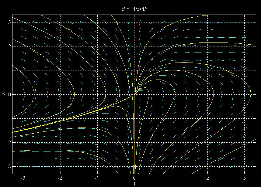
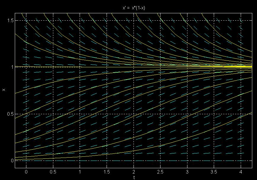
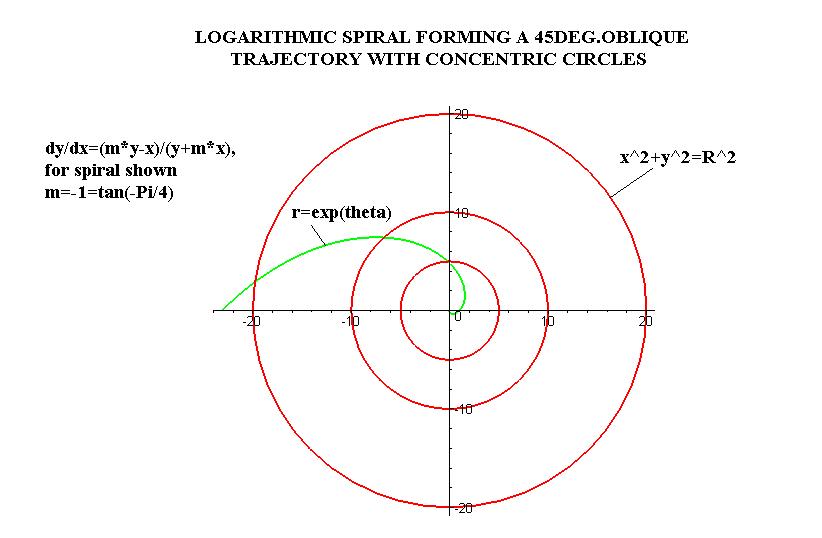
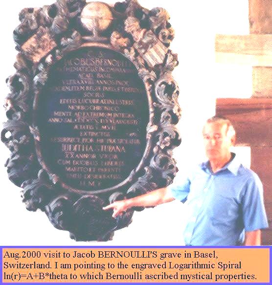
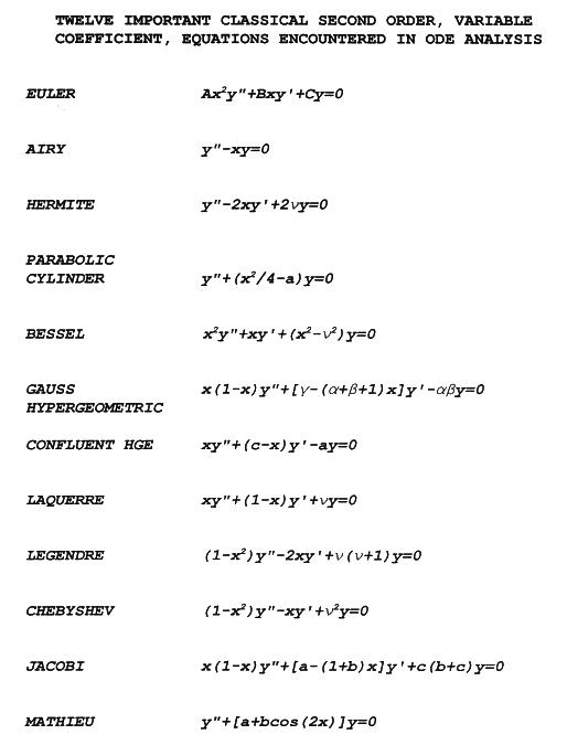
![AIRY FUNCTIONS OF THE FIRST [Ai(x)] AND SECOND [Bi(x)] KIND:](http://www2.mae.ufl.edu/%7Euhk/airy1.JPG)
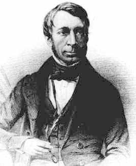
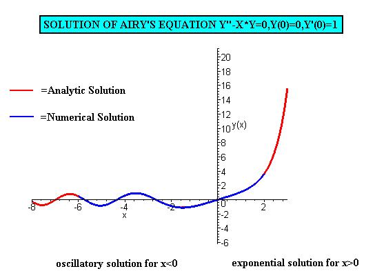
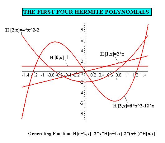
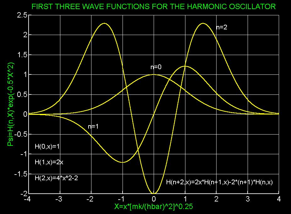
![BESSEL FUNCTIONS OF THE FIRST KIND[J(n,x)]:](http://www2.mae.ufl.edu/%7Euhk/bessJ.JPG)
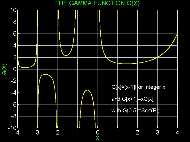
![BESSEL FUNCTIONS OF THE SECOND KIND [Y(n,x)]:](http://www2.mae.ufl.edu/%7Euhk/ybess.jpg)
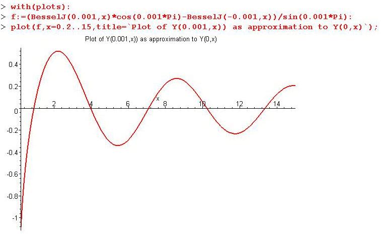
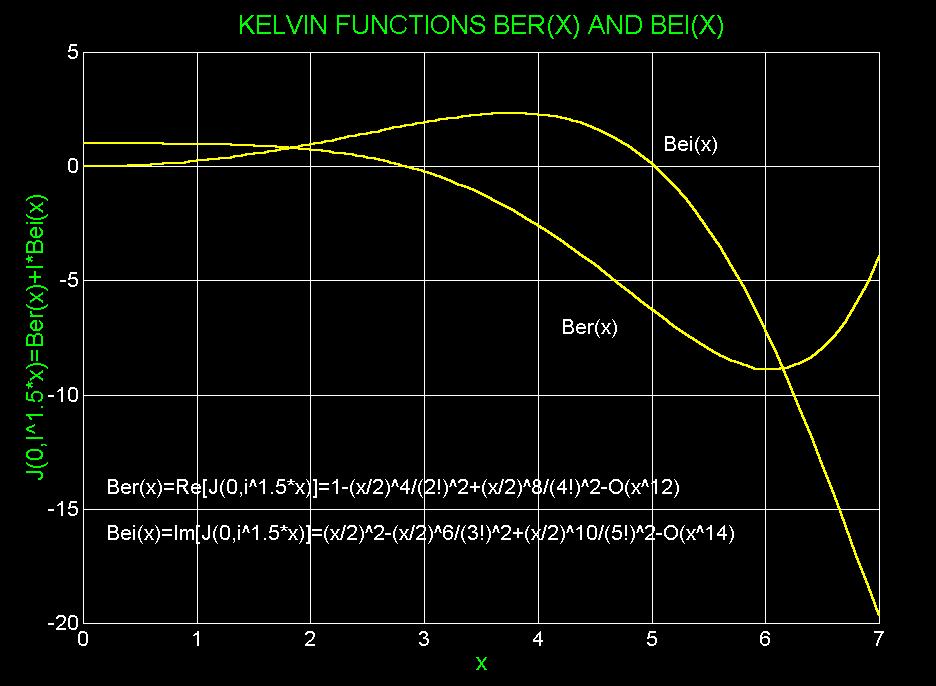
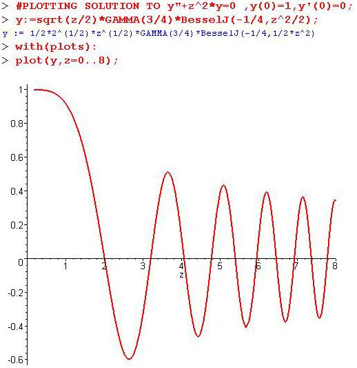
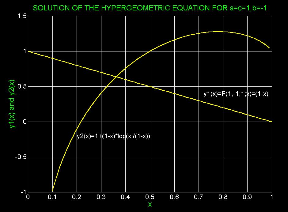
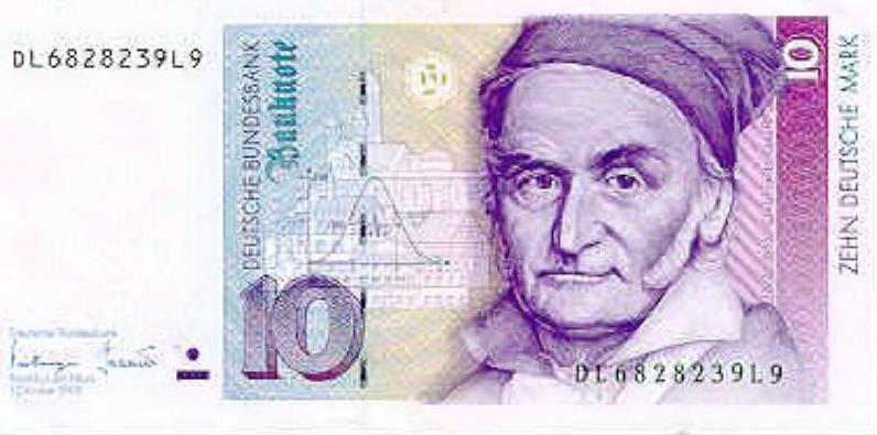
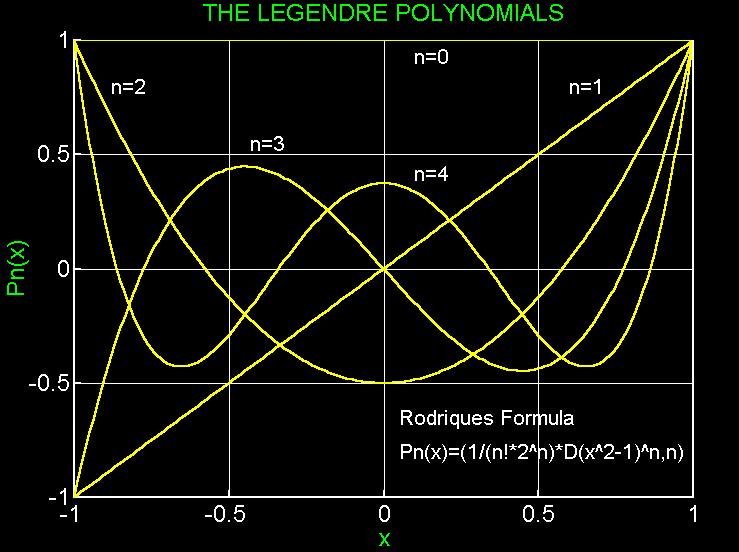
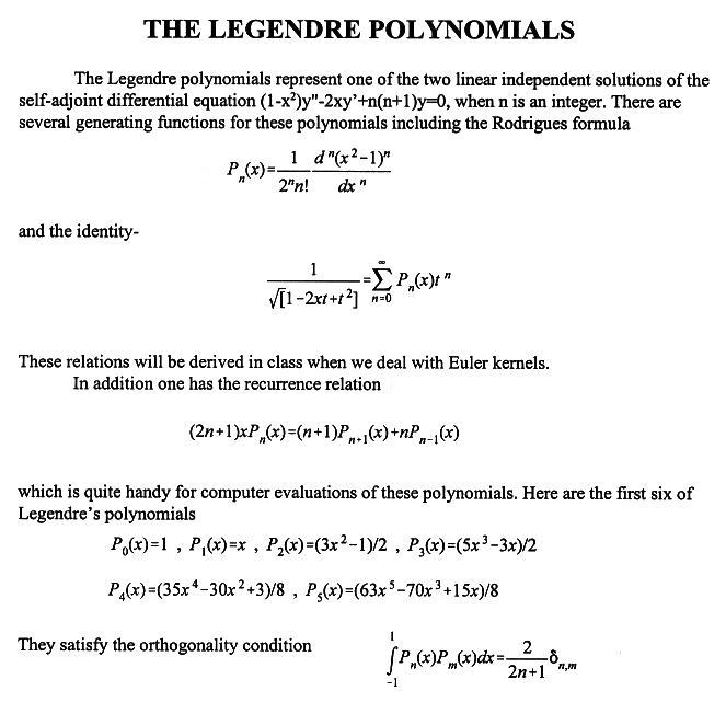
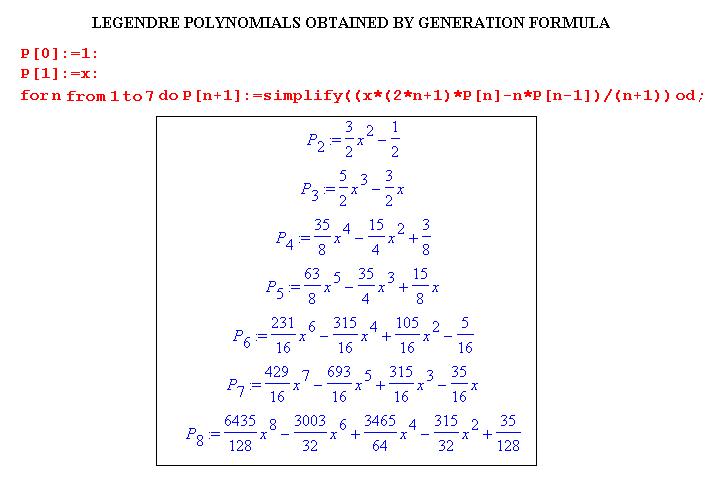
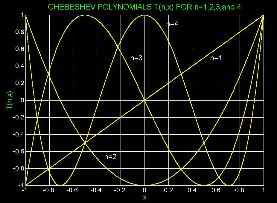
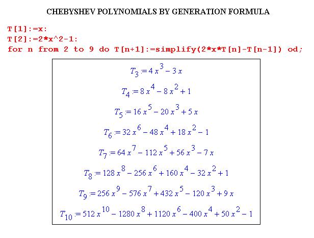
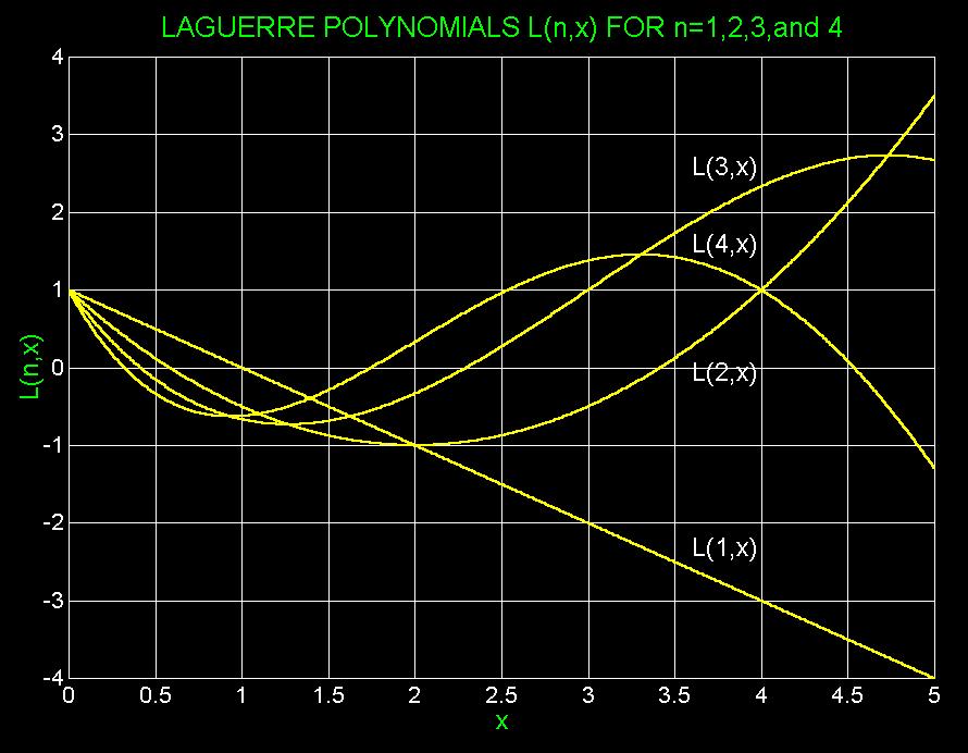
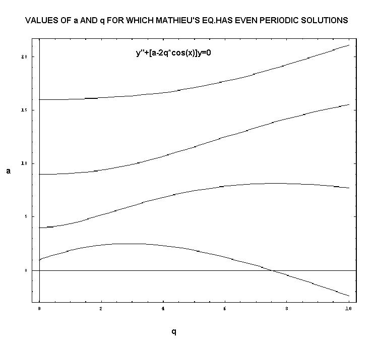
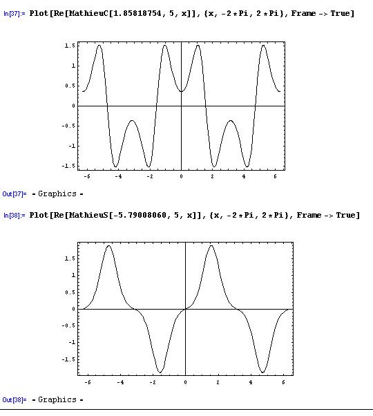
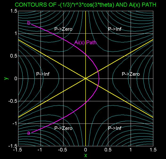
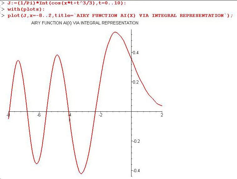
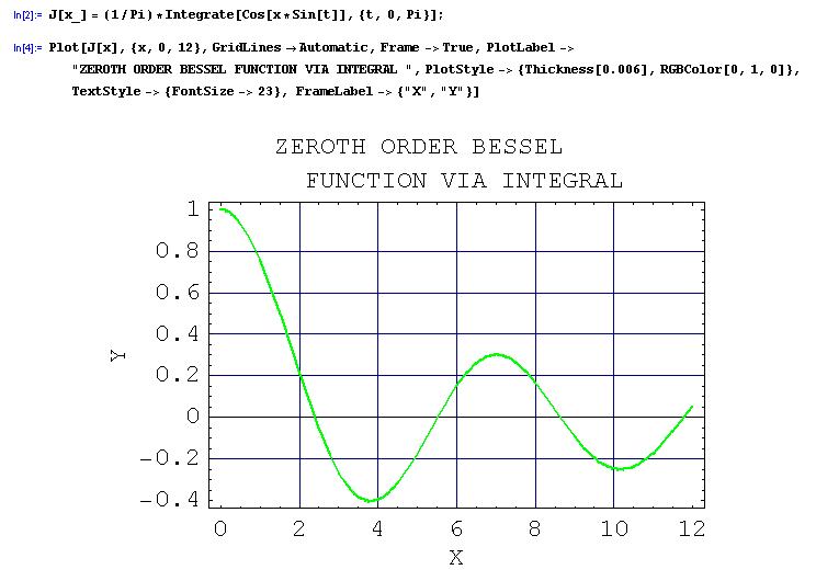
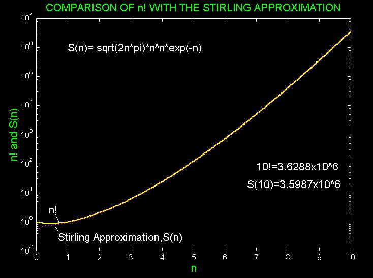
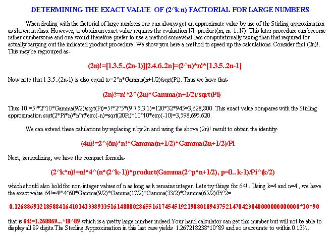
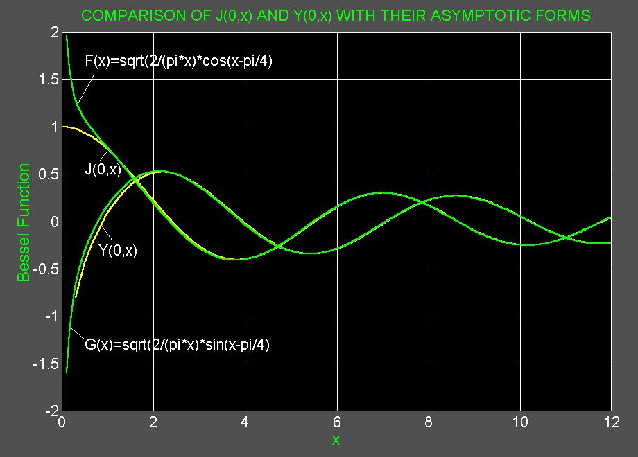
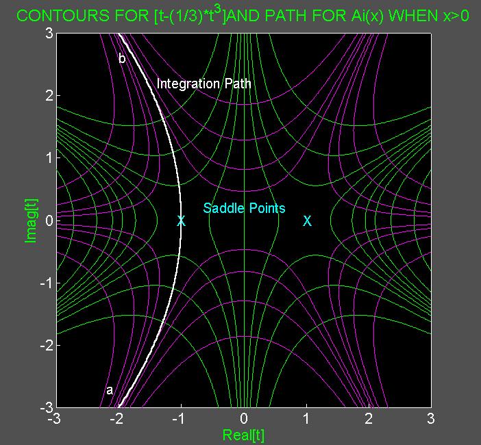
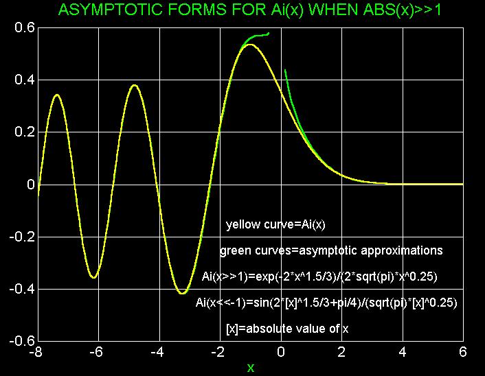
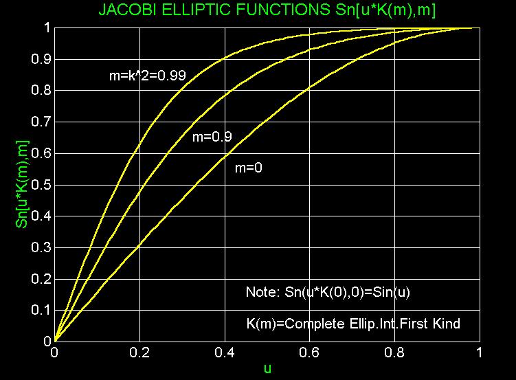
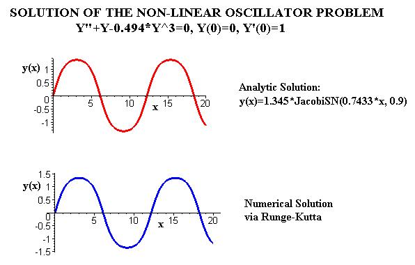
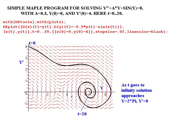
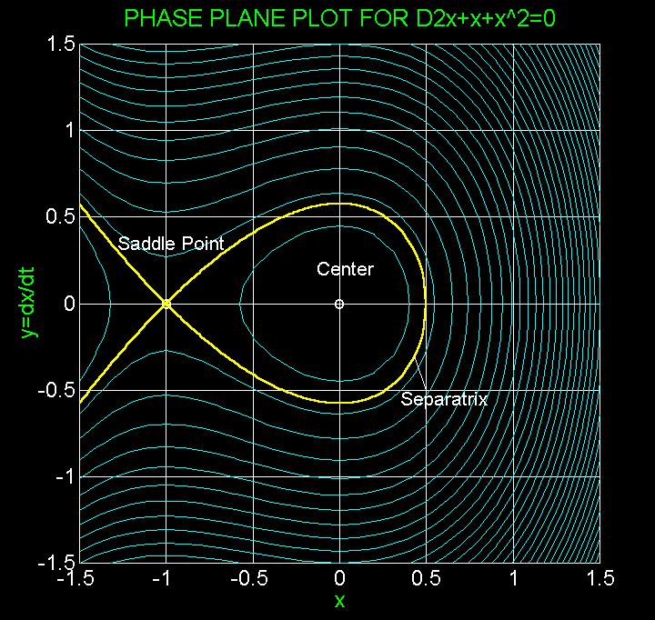
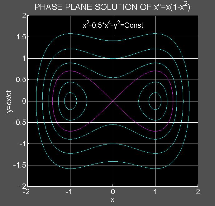
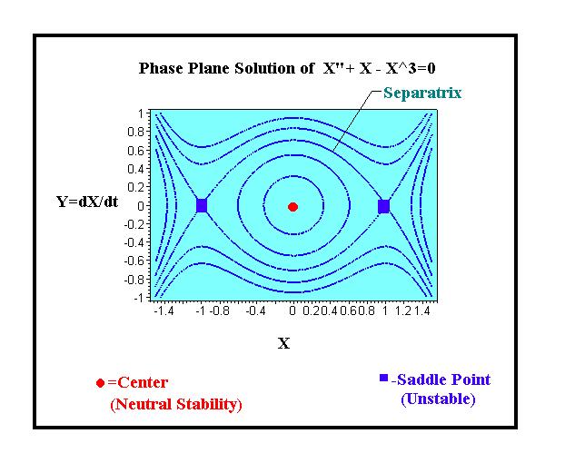
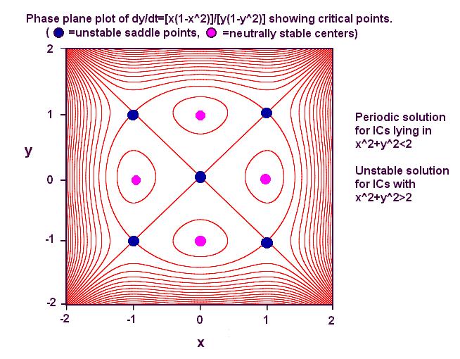
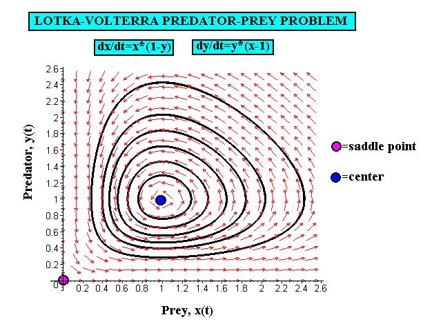
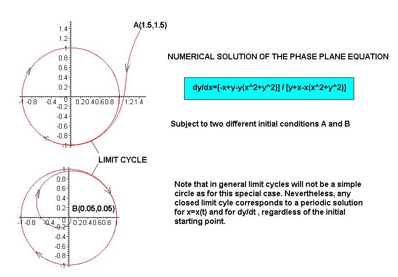
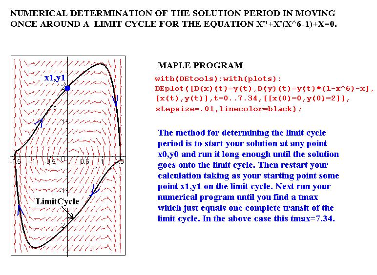
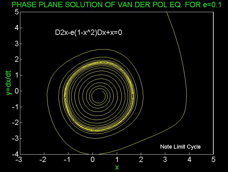
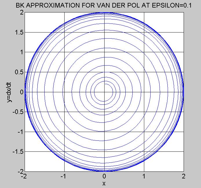
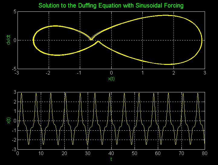
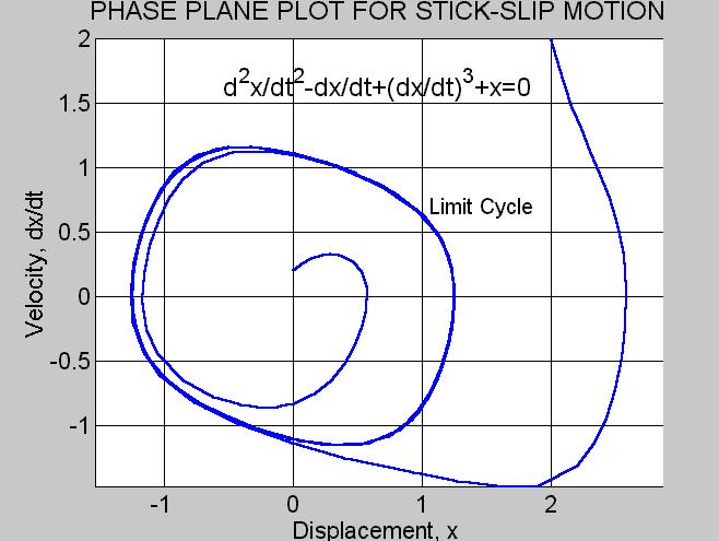
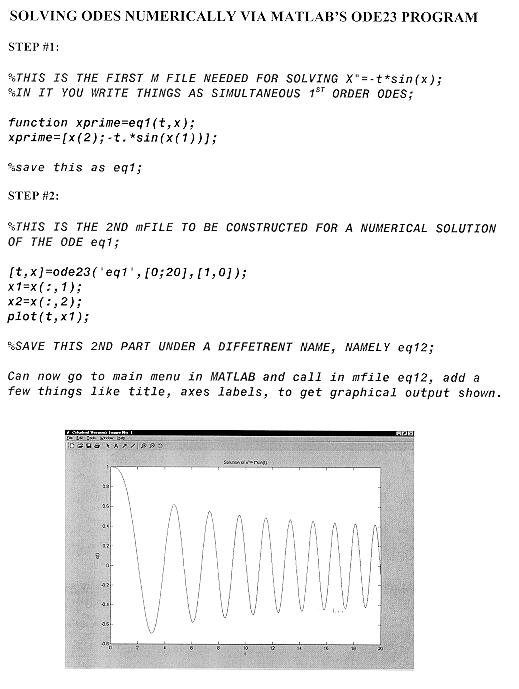
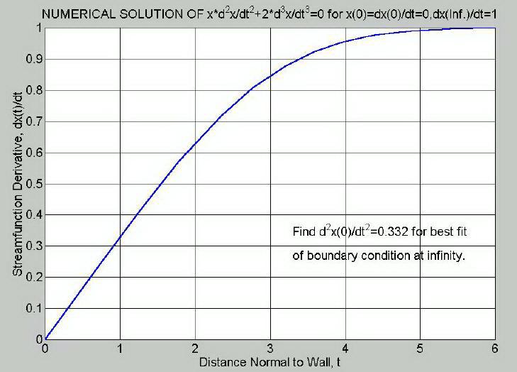
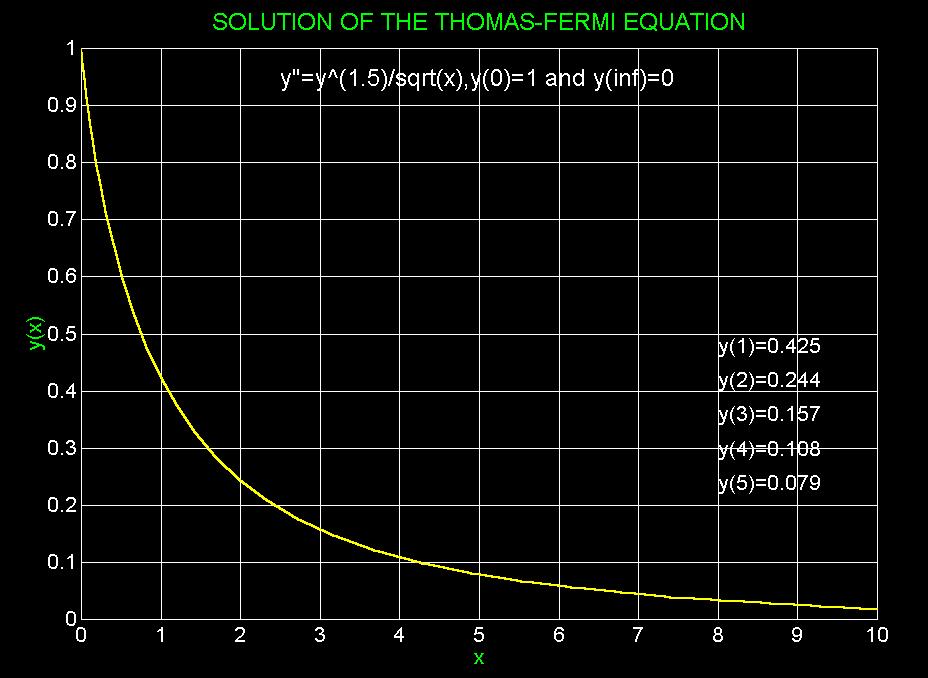
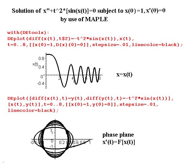
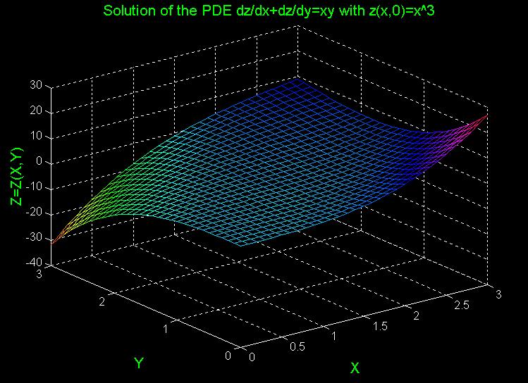
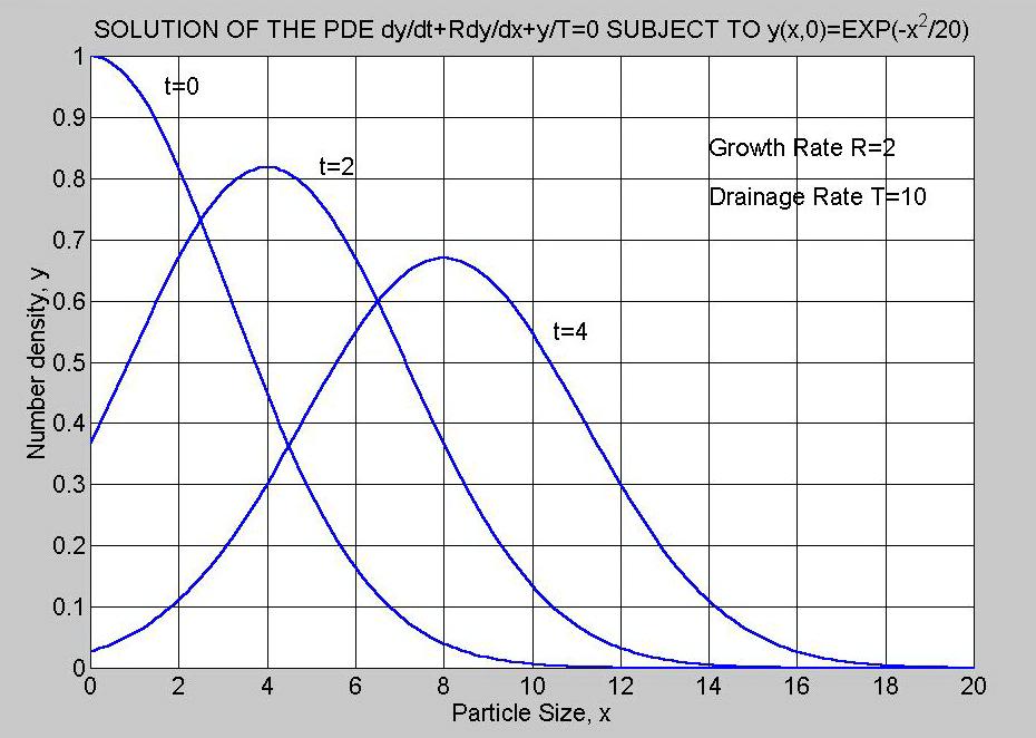
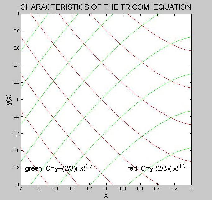
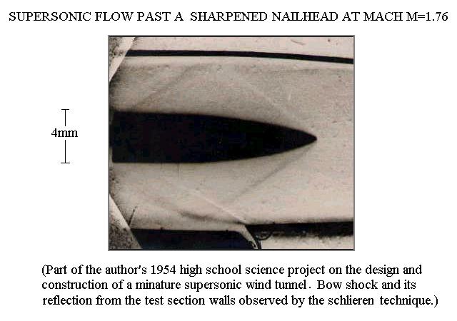
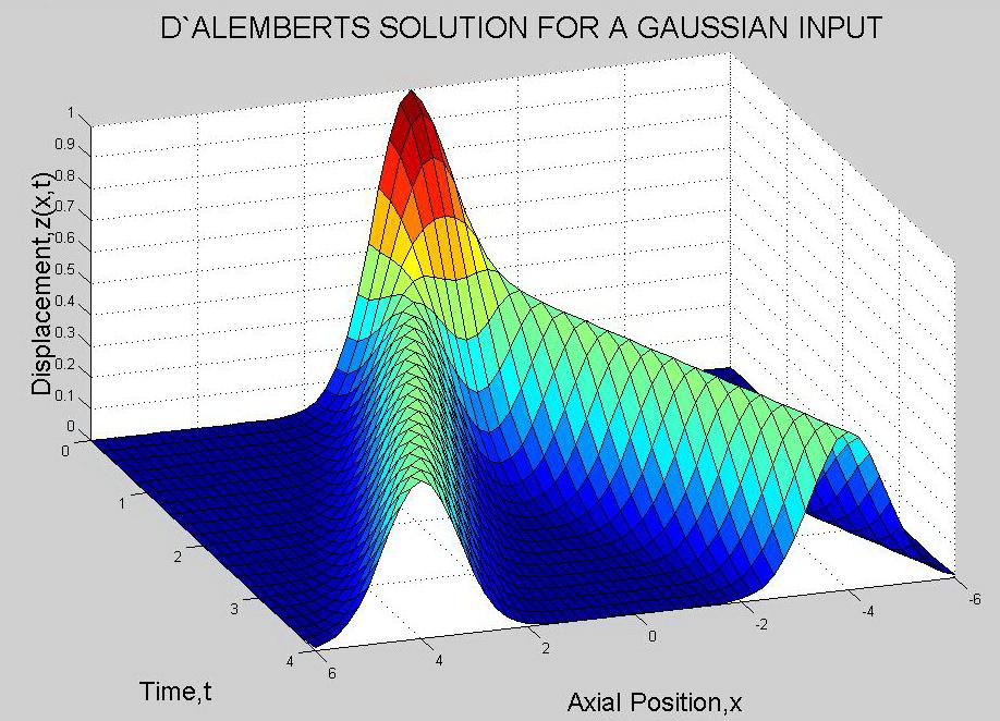
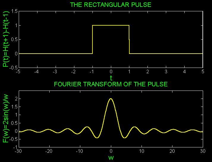
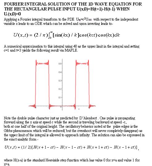
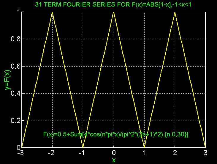
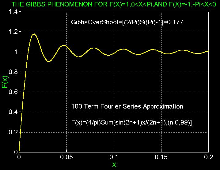
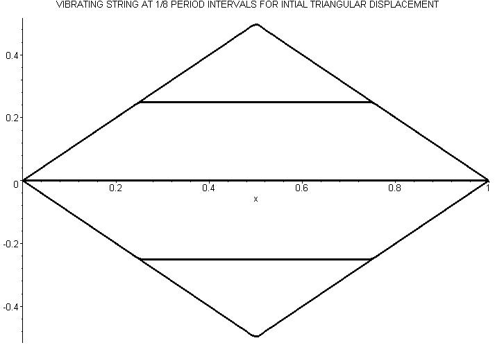
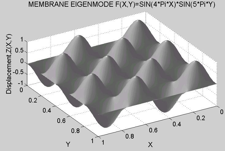
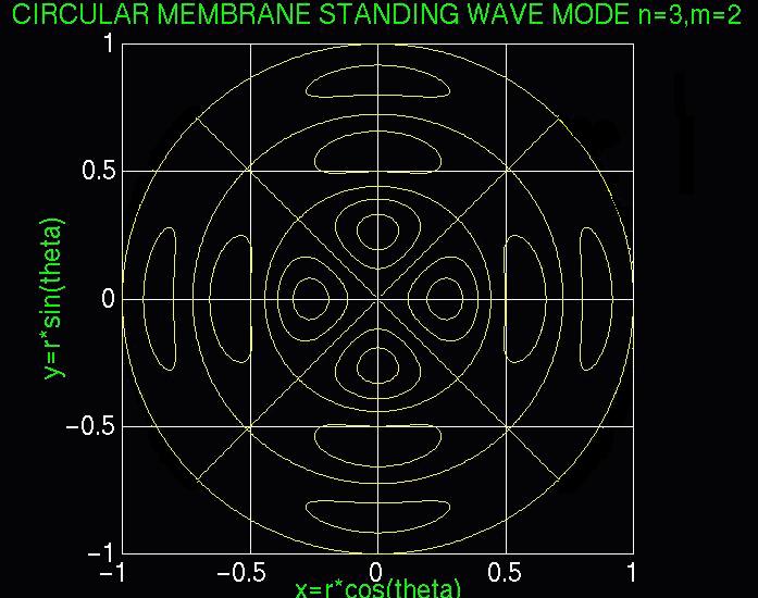
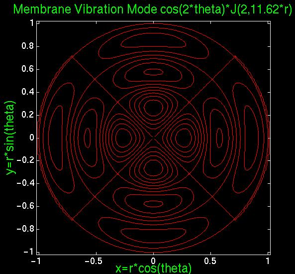
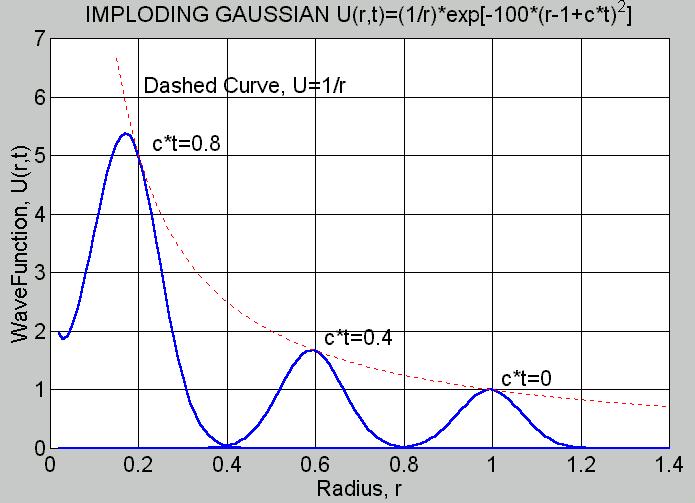
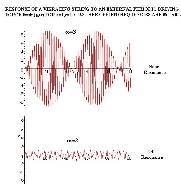
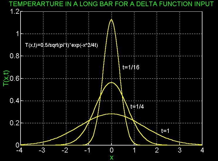
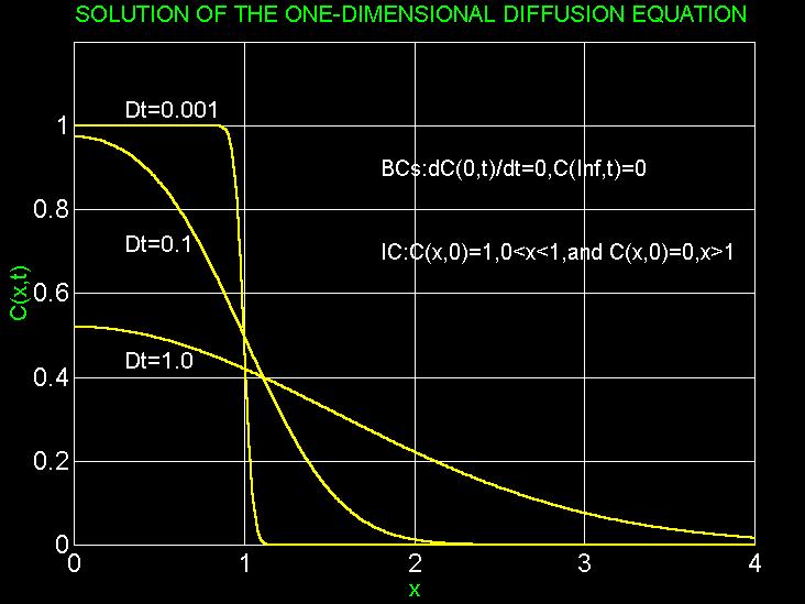
![ERROR FUNCTION [ERF(X)] AND ITS COMPLEMENT [ERFC(X)]:](http://www2.mae.ufl.edu/%7Euhk/Erf.jpg)
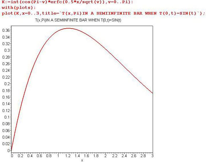
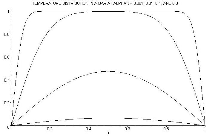
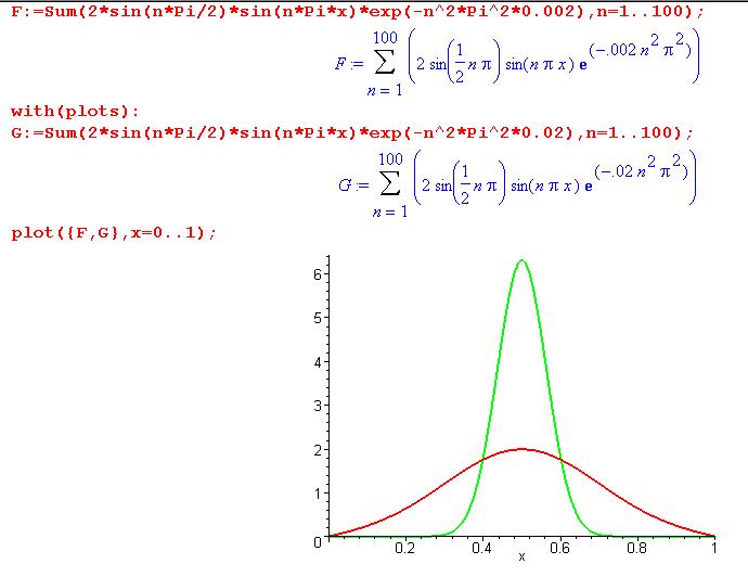
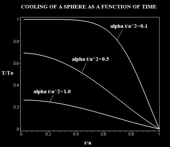
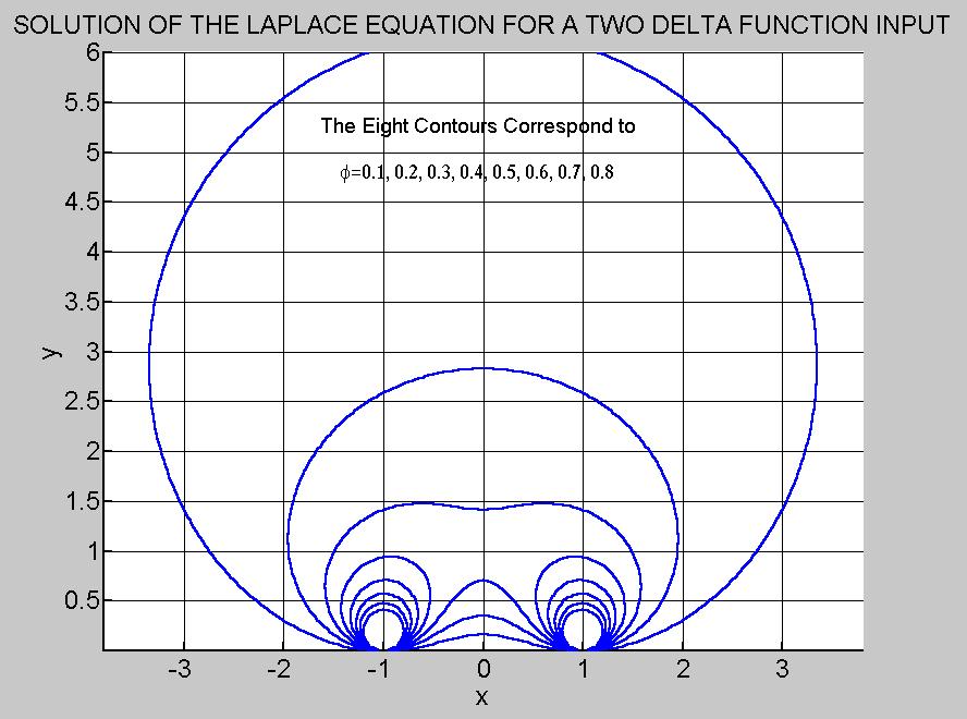
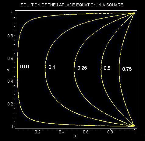
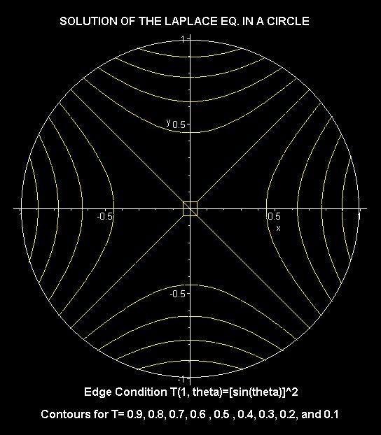
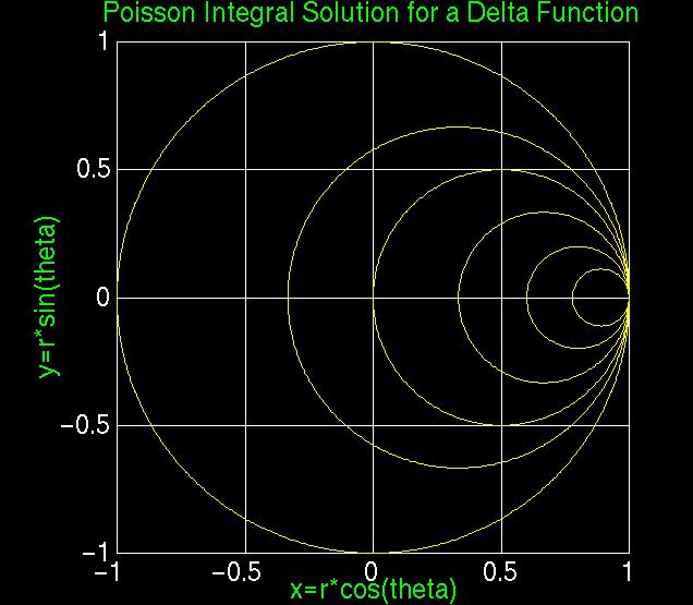
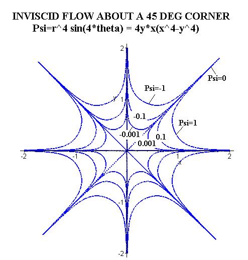
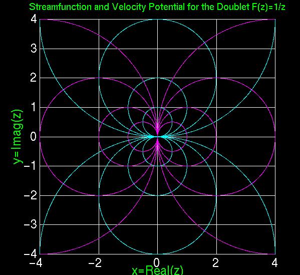
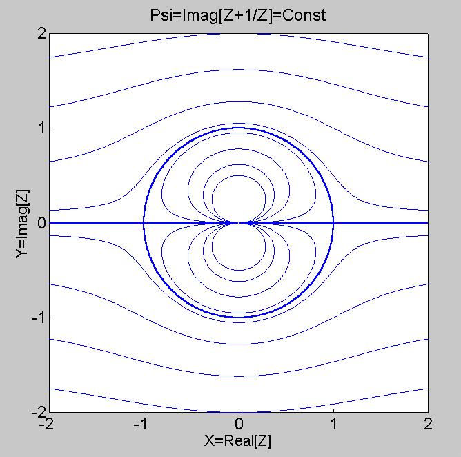
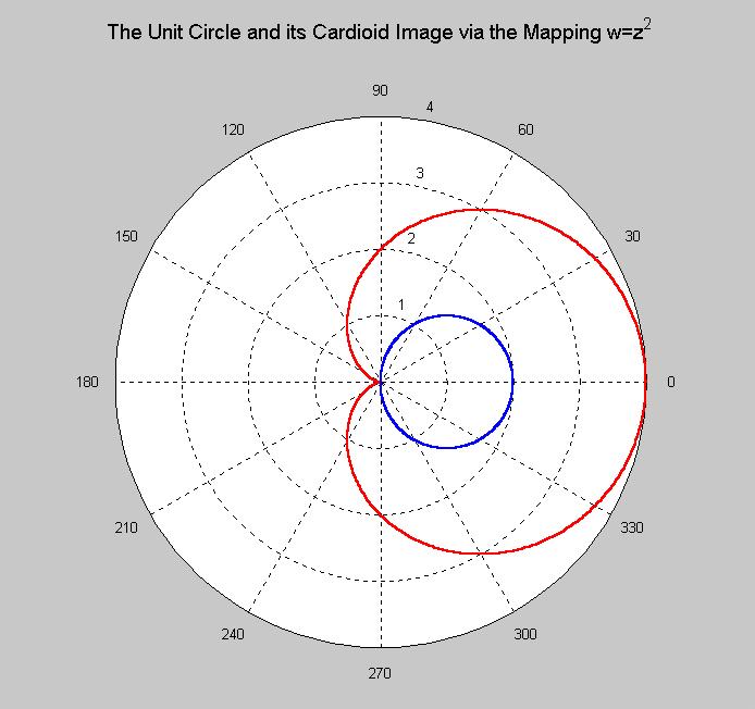
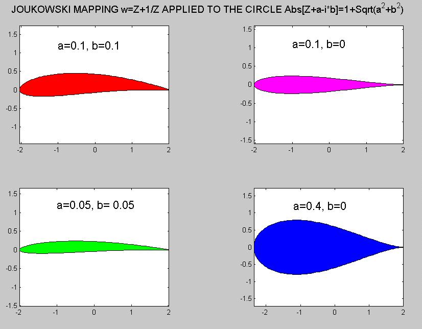
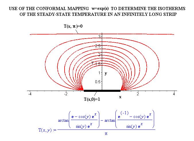
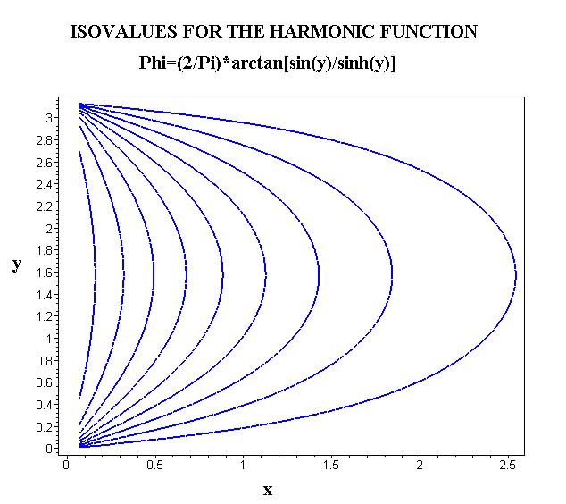
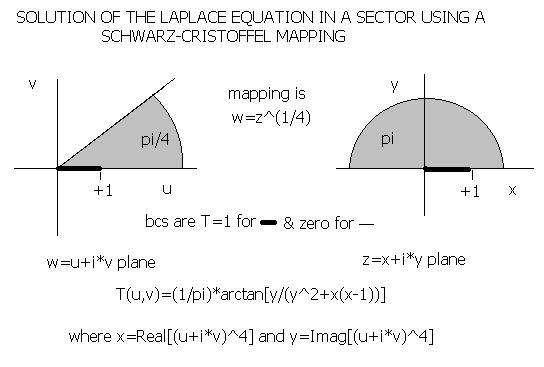
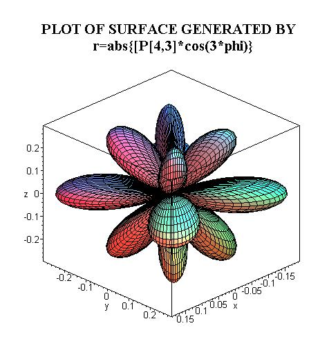
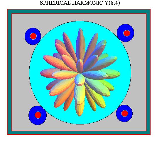
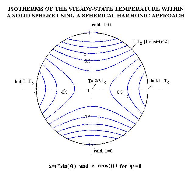
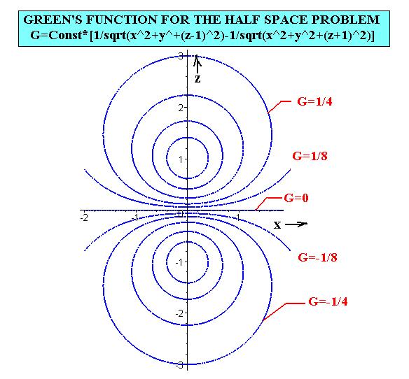
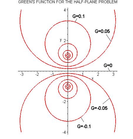
![SPERICAL BESSEL FUNCTIONS OF THE FIRST KIND [j(n,x)]:](http://www2.mae.ufl.edu/%7Euhk/sphj.JPG)
![SPERICAL BESSEL FUNCTIONS OF THE SECOND KIND[n(n,x)]:](http://www2.mae.ufl.edu/%7Euhk/sphn.JPG)
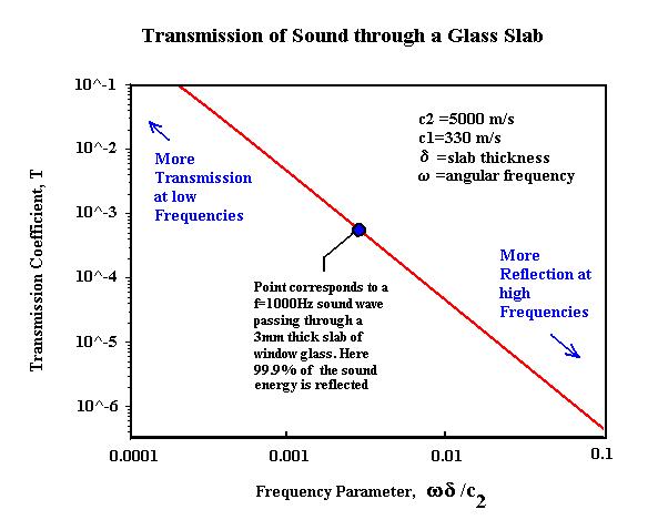
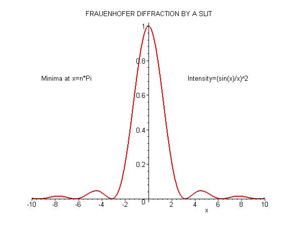
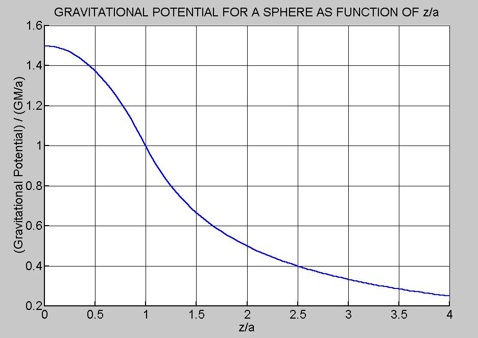
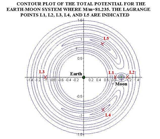
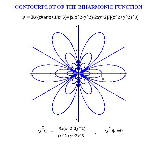
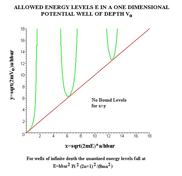
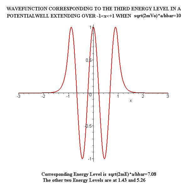
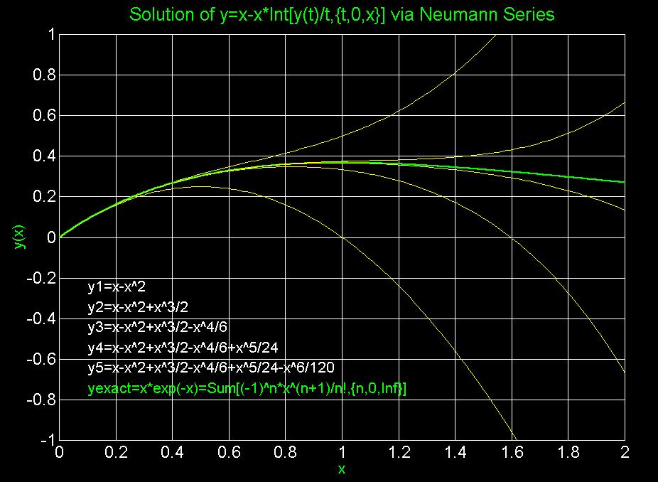
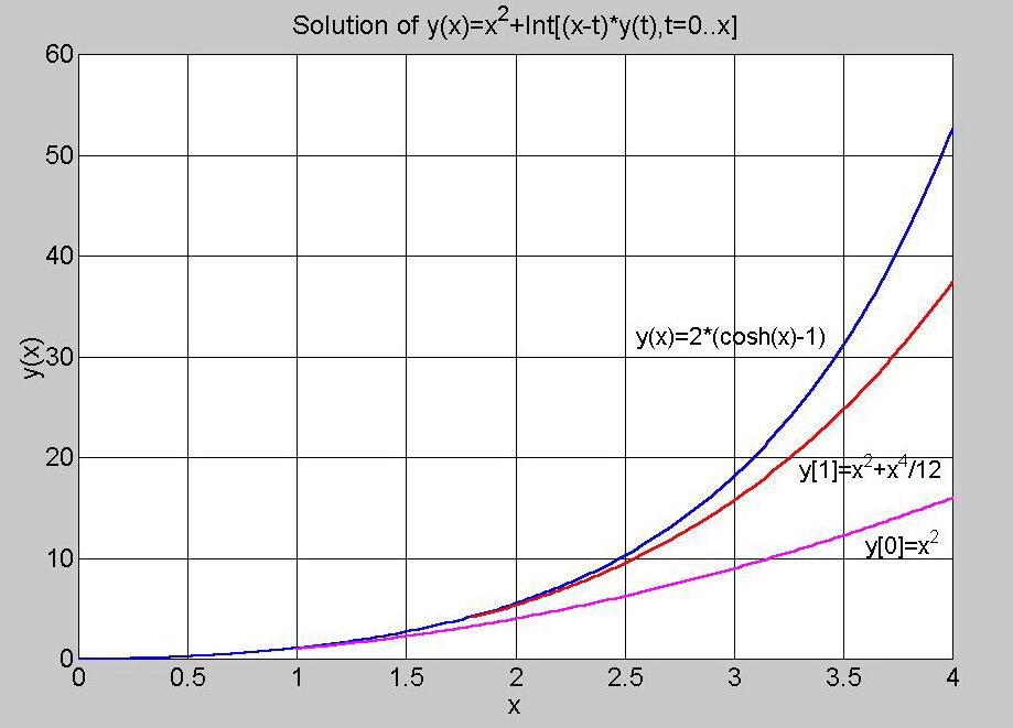
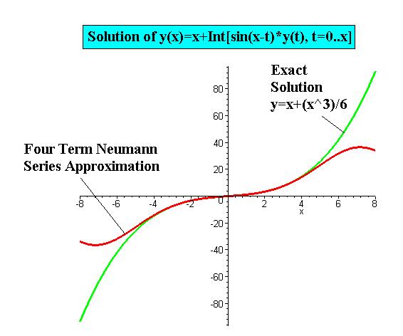
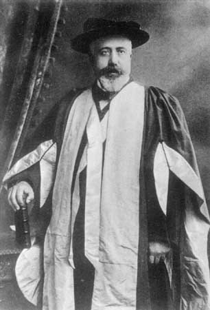
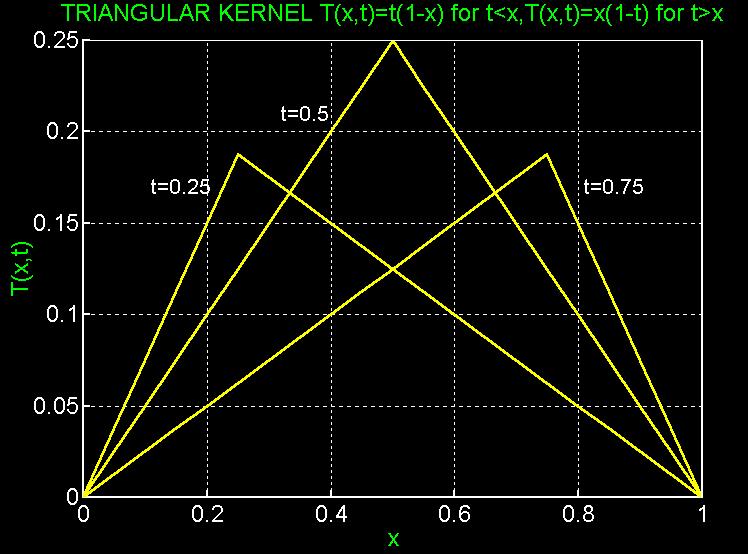
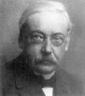
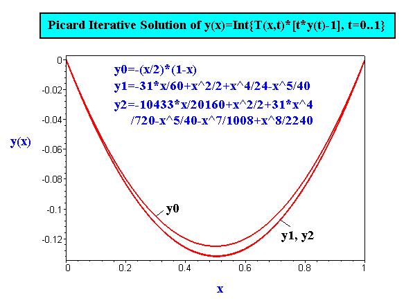
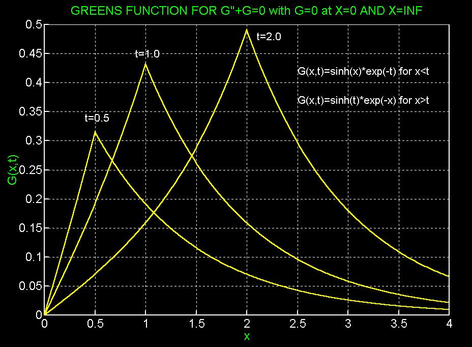
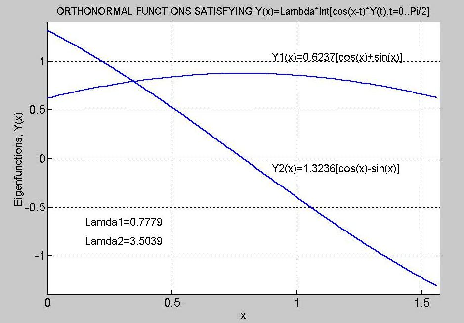
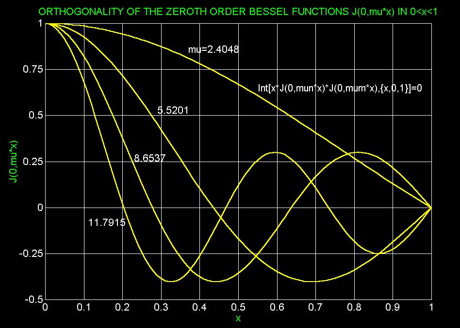
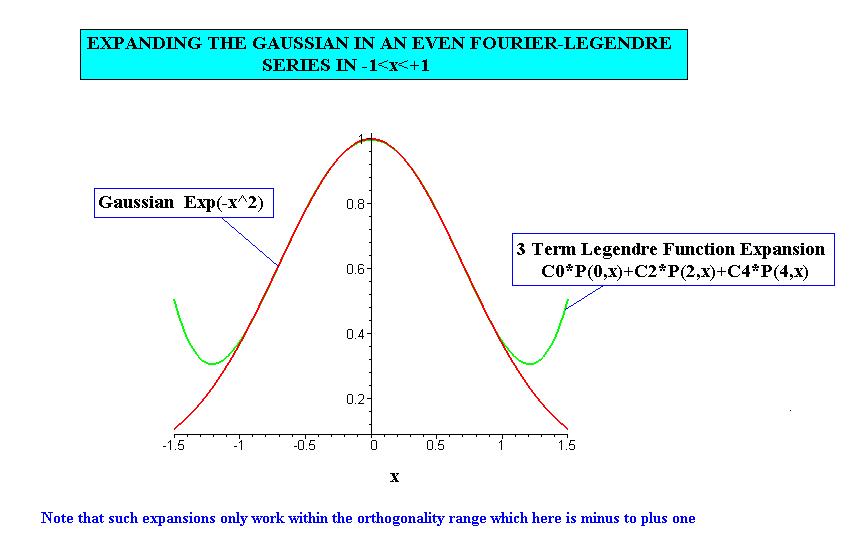
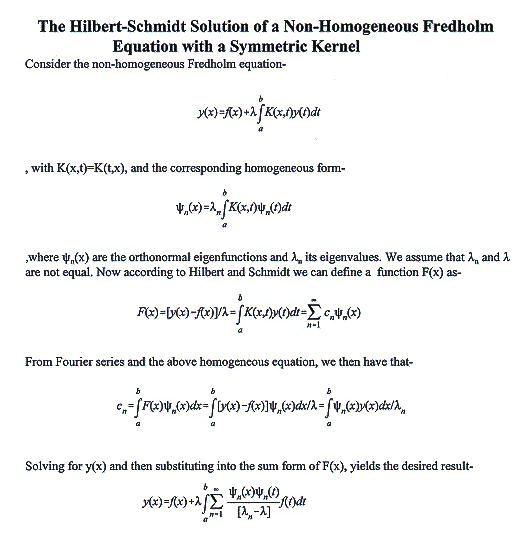
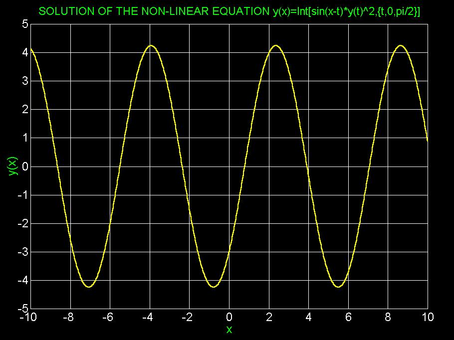
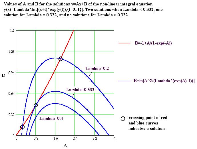
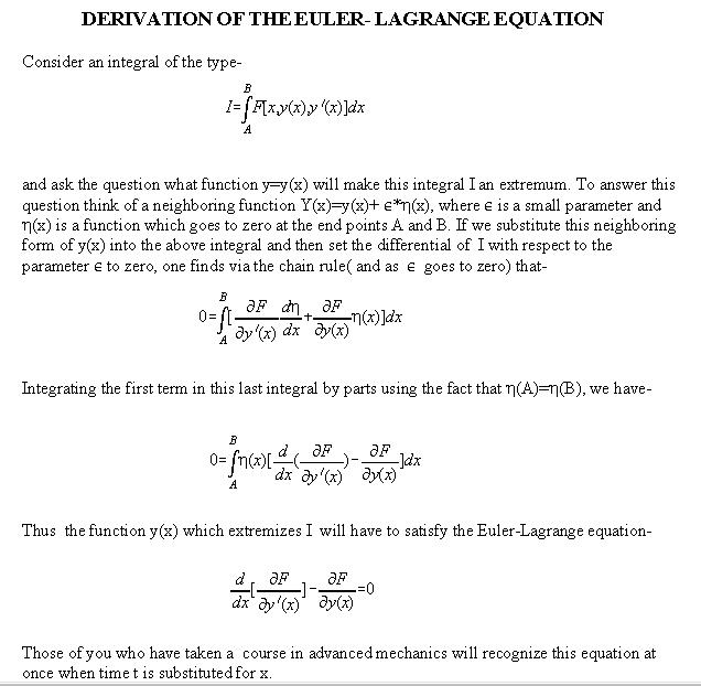
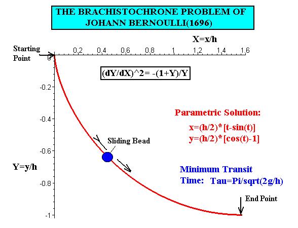
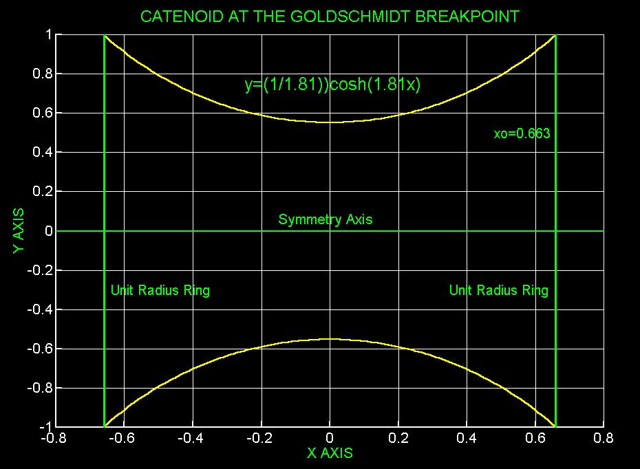
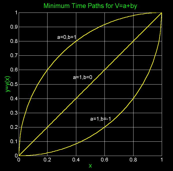
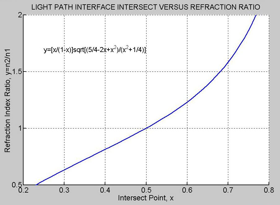
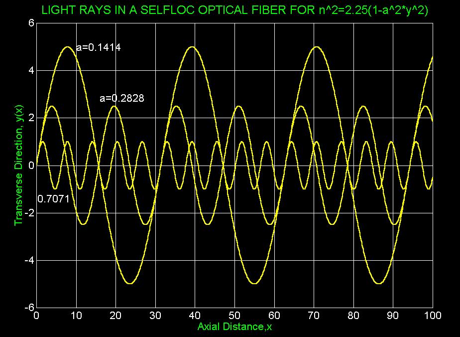
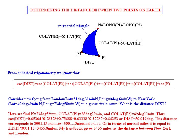
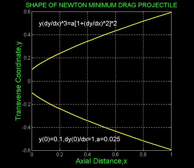
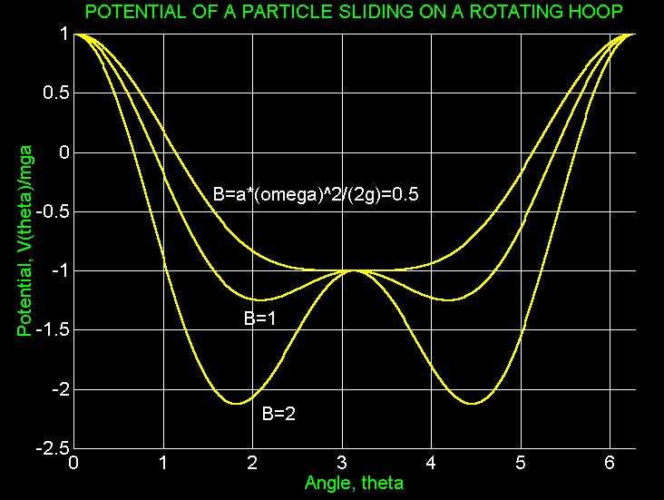
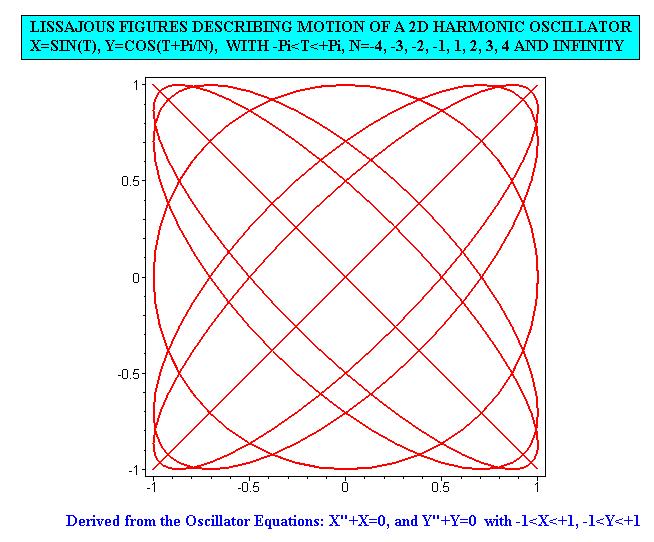
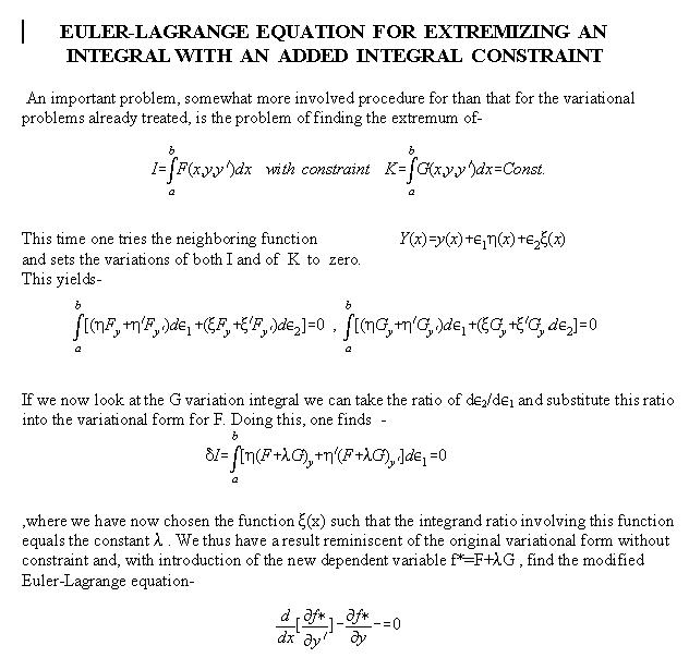
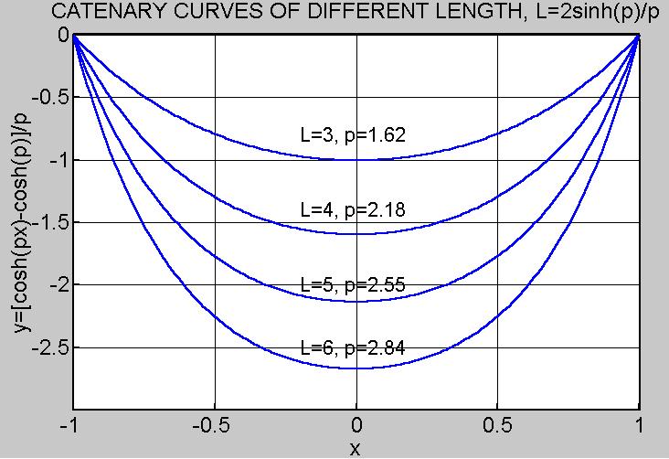
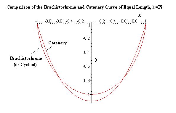
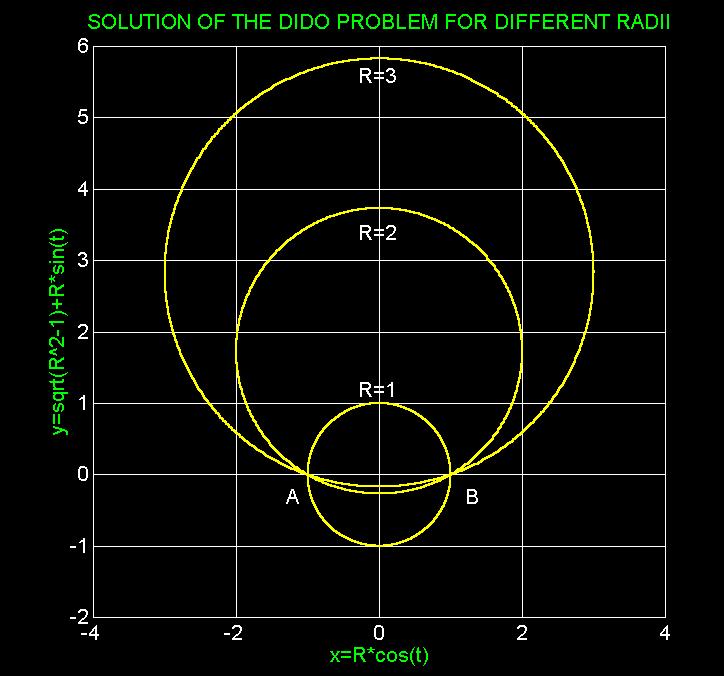
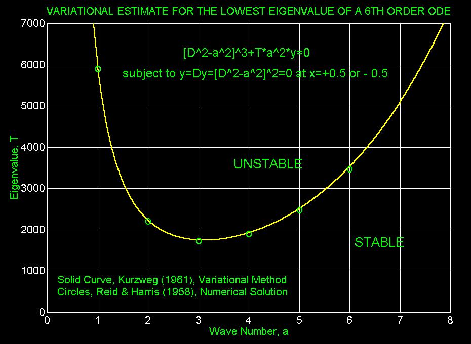
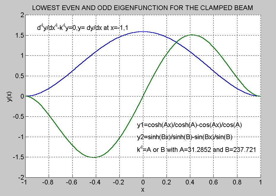
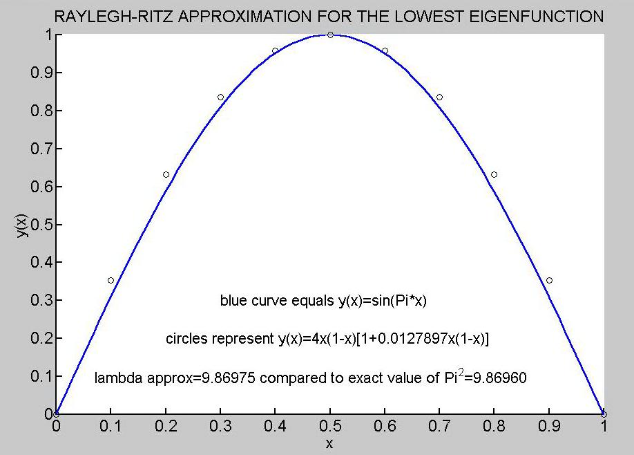
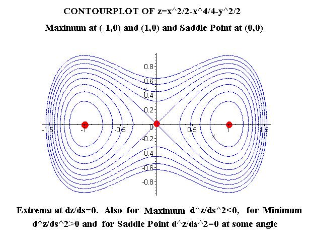